![[Update] I tried out anomaly detection with the new FIXED mode in AWS Glue Data Quality](https://images.ctfassets.net/ct0aopd36mqt/wp-thumbnail-545ba5dfbc8fa4c7760dd9872ef835f9/665944e579f487b4434cb289305767b3/aws-glue?w=3840&fm=webp)
[Update] I tried out anomaly detection with the new FIXED mode in AWS Glue Data Quality

This page has been translated by machine translation. View original
This is Ishikawa from the Cloud Business Division. Anomaly Detection in AWS Glue Data Quality ETL jobs is now available at no additional charge, and a new observation mode (FIXED) has been added to reduce false positives, so I tried it out from the management console.
AWS Glue Data Quality's anomaly detection is a feature where a machine learning model learns statistics collected by rules and analyzers (such as row count and completeness) as a time series and detects values that deviate from the predicted range as anomalies. Previously, anomaly detection in ETL jobs incurred an additional charge of 1 DPU per statistic, but with this update, it can now be used at no additional charge.
Along with this, a new observation mode has been introduced. The conventional prediction (LINEAR mode) extrapolates linear trends, which made it prone to false anomalies when execution intervals are irregular or when data has no clear trend. The new FIXED mode addresses this issue by predicting with a constant baseline.
What is AWS Glue Data Quality Anomaly Detection
AWS Glue Data Quality is a feature that enables serverless measurement, monitoring, and improvement of data quality. In addition to rule-based checks, it provides machine learning-powered anomaly detection.
Anomaly detection learns patterns of statistical values such as row count (RowCount) from past executions and detects deviations by taking into account seasonality and trends. It is characterized by the ability to detect "unusual" data changes that cannot be captured by rules using fixed thresholds, without writing any code.
Update Contents
The main changes in this update are as follows.
- Anomaly detection in ETL jobs is now available at no additional charge: You can now monitor data quality anomalies across all AWS Glue pipelines without worrying about cost
- Introduction of a new observation mode: A new observation mode has been added to reduce false anomaly detection
- Improved prediction method: Using a constant baseline instead of a linear trend avoids excessive extrapolation of trends, resulting in more accurate alerts and reduced noise
- Improved handling of irregular data arrival intervals: Even in notebook-based and exploratory workflows, cases where data arrives at irregular intervals can now be handled appropriately
The new observation mode is said to be particularly useful in the following cases.
- Exploratory data analysis
- Datasets with flat or random patterns
- Workloads without predictable trends
- Data quality checks with non-fixed execution schedules or execution in interactive environments like notebooks
Because conventional anomaly detection predicts future values from past trends, it sometimes detected actually non-problematic changes as anomalies when execution intervals were irregular or when data had no clear trend. This improvement reduces such noise, making it easier to focus on anomalies that truly need to be addressed.
What are Anomaly Detection Observation Modes (LINEAR / FIXED)
According to the official documentation, there are two observation modes available for anomaly detection.
- LINEAR (default): Learns data trends and seasonality and extrapolates future values for prediction. Suitable for regularly scheduled execution where data has a consistent increasing/decreasing trend or weekly/daily periodicity
- FIXED: Treats all data points as equally spaced regardless of execution intervals, and establishes a constant baseline from observations for prediction. Suitable for data with flat or randomly varying patterns, irregular interval execution, and exploratory analysis in notebooks
Anomaly detection requires a minimum of 3 data points, and from subsequent runs, predicted values are compared with actual values.
In ETL jobs, observations.mode is specified in the additional_options of EvaluateDataQuality. For evaluation runs on tables in the AWS Glue Data Catalog, it is specified in the ObservationMode field of AdditionalRunOptions. If not specified, it operates in LINEAR mode.
In the AWS Glue Studio visual editor, you can enable anomaly detection and add analyzers from the "Anomaly detection" tab of the Evaluate Data Quality node, but specifying the observation mode is done via script-side options. Therefore, I will create the job using the Script editor this time.
Try It Out
Prerequisites
- IAM role for Glue job execution (Glue service role including read access to S3)
- Verification environment: ap-northeast-1, AWS Glue 5.1 (G.1X worker × 2)
Preparing Test Data
I prepared 5 generations of sales-like CSV files where only the row count changes. Generations 1 through 4 vary randomly around 100 rows (100 → 102 → 97 → 101 rows), and only generation 5 is significantly reduced to 30 rows to plant an "anomaly."
generate_and_upload.py
import csv
import random

random.seed(42)
products = ["apple", "banana", "cherry", "grape", "orange"]
row_counts = {1: 100, 2: 102, 3: 97, 4: 101, 5: 30}

for gen, n in row_counts.items():
    with open(f"sales_gen{gen}.csv", "w", newline="") as f:
        w = csv.writer(f)
        w.writerow(["order_id", "product", "quantity", "price"])
        for i in range(1, n + 1):
            w.writerow([
                f"G{gen}-{i:04d}",
                random.choice(products),
                random.randint(1, 9),
                random.randint(100, 2000),
            ])
The generated CSV contains content like the following.
order_id,product,quantity,price
G1-0001,apple,1,1618
G1-0002,cherry,4,557
G1-0003,banana,2,1485
G1-0004,orange,2,1309
G1-0005,grape,1,161
Open the Amazon S3 console and create a verification bucket from "Create bucket." This time, I used the name blog-tryit-20260810 with the region set to ap-northeast-1.
Open the created bucket, create an input folder using "Create folder." Then create folders gen1 through gen5 inside input, and upload the corresponding generation's CSV to each folder with the name sales.csv.
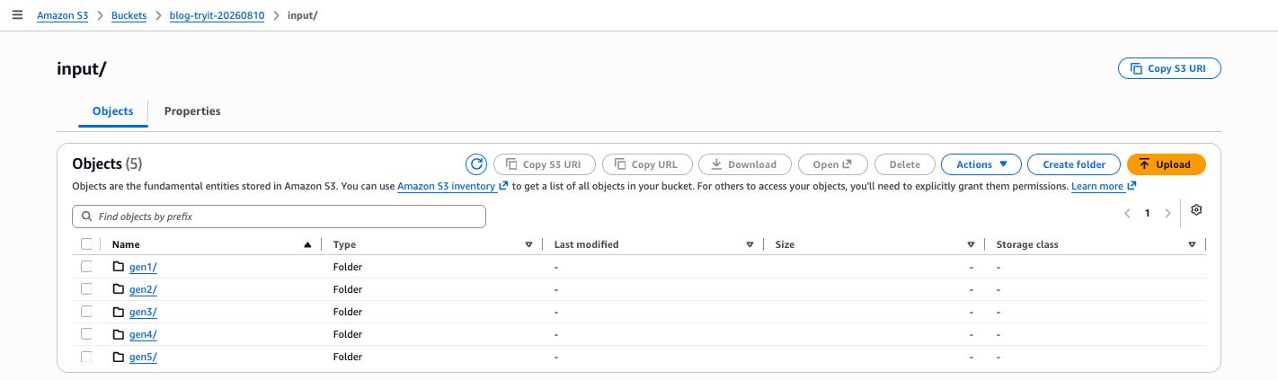
The object list after uploading is as follows. You can see that only the 5th generation file has a smaller size.
| Key | Size |
|---|---|
| input/gen1/sales.csv | 2,245 bytes |
| input/gen2/sales.csv | 2,292 bytes |
| input/gen3/sales.csv | 2,177 bytes |
| input/gen4/sales.csv | 2,271 bytes |
| input/gen5/sales.csv | 702 bytes |
Creating a Glue Job with FIXED Mode Specified
Open "ETL jobs" from the left navigation of the AWS Glue console, and select "Script editor." Select "Spark" for Engine and "Start fresh" for Options, then click "Create script."
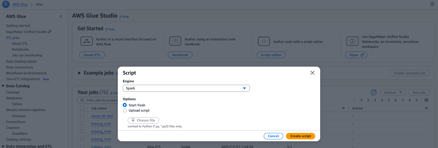
Paste the following PySpark script into the script editor. The key point is specifying observations.mode: FIXED in the additional_options of EvaluateDataQuality. The analyzers collect RowCount (row count) and Completeness of the product column.
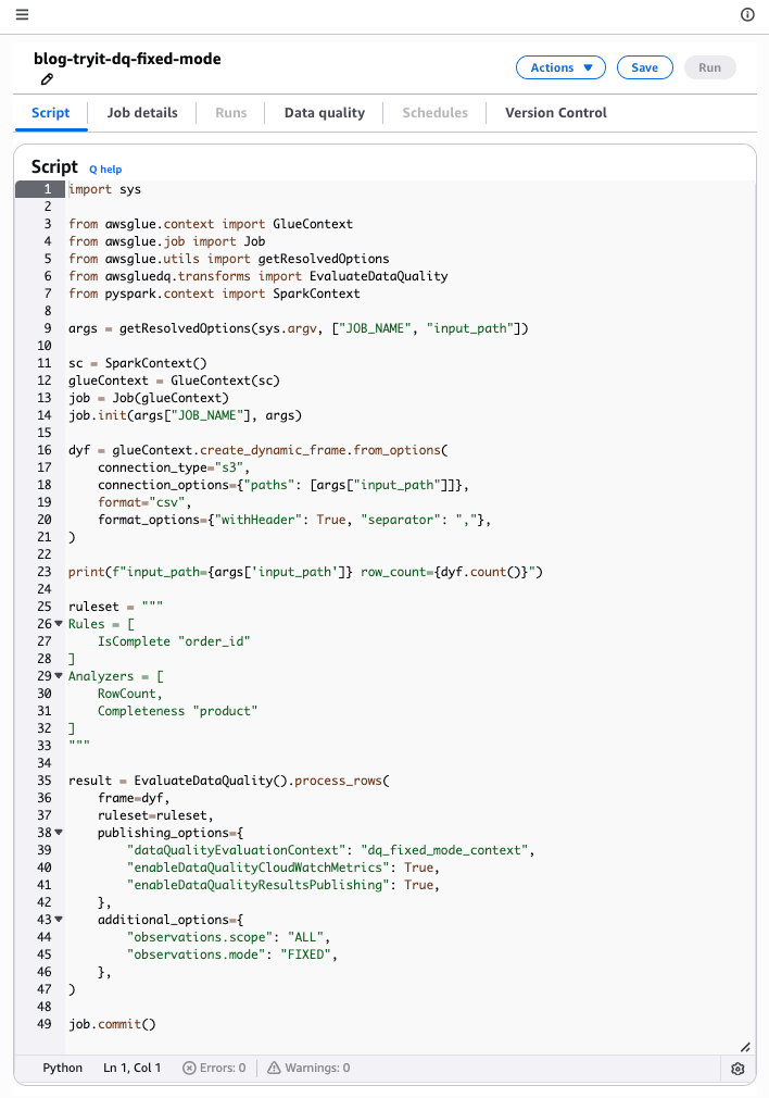
First, the data quality ruleset is written in DQDL (Data Quality Definition Language). The content I specified this time is as follows.
ruleset = """
Rules = [
    IsComplete "order_id"
]
Analyzers = [
    RowCount,
    Completeness "product"
]
"""
Rules and Analyzers have different roles.
| Section | Role |
|---|---|
Rules |
Writes expected conditions and judges pass/fail (PASS / FAIL). Results are reflected in the Data quality score |
Analyzers |
Does not judge pass/fail, only collects statistics. Allows monitoring of columns where thresholds cannot be determined |
The content specified this time is as follows.
| Description | Section | Content |
|---|---|---|
IsComplete "order_id" |
Rules | Verifies that the order_id column has no empty values or NULLs |
RowCount |
Analyzers | Collects the row count of the dataset |
Completeness "product" |
Analyzers | Collects the completeness rate of the product column |
Anomaly detection works on the time series of statistics collected here. The key point is that RowCount is specified as an analyzer since we want to detect a sudden decrease in row count this time. Other statistics that can be specified with analyzers include Completeness, Uniqueness, Mean, Sum, StandardDeviation, Entropy, DistinctValuesCount, UniqueValueRatio, and more. If there are no columns where thresholds can be determined, you can also write only Analyzers with Rules left empty.
Note that according to the official documentation, even if both a Rule and an Analyzer are specified for the same column, statistics are collected only once.
The statistics collected by this ruleset are 3: Column.order_id.Completeness from IsComplete "order_id", Dataset.*.RowCount from the analyzer, and Column.product.Completeness. The fact that "Statistics gathered" shows 3 in the "Data quality" tab later refers to these 3 items.
The anomaly detection configuration is consolidated in the EvaluateDataQuality call. Extracting the relevant part is as follows.
result = EvaluateDataQuality().process_rows(
    frame=dyf,
    ruleset=ruleset,
    publishing_options={
        "dataQualityEvaluationContext": "dq_fixed_mode_context",
        "enableDataQualityCloudWatchMetrics": True,
        "enableDataQualityResultsPublishing": True,
    },
    additional_options={
        "observations.scope": "ALL",
        "observations.mode": "FIXED",
    },
)
The role of each argument is as follows.
| Argument | Role |
|---|---|
frame |
The DynamicFrame to be evaluated. This time, one created from the CSV in S3 is passed |
ruleset |
The ruleset written in DQDL. Rules judges pass/fail, and Analyzers only collects statistics without judging pass/fail |
publishing_options |
Specifies how evaluation results are published |
additional_options |
Specifies the behavior of anomaly detection |
Each key in publishing_options corresponds to a field in the API's DQResultsPublishingOptions.
| Key | Corresponding API field | Role |
|---|---|---|
dataQualityEvaluationContext |
EvaluationContext |
Context name for grouping evaluation results |
enableDataQualityCloudWatchMetrics |
CloudWatchMetricsEnabled |
Enables CloudWatch metrics for data quality results |
enableDataQualityResultsPublishing |
ResultsPublishingEnabled |
Enables publishing of evaluation results |
The name specified for dataQualityEvaluationContext appears as-is in the console screen confirmed later. Since I specified dq_fixed_mode_context this time, the ruleset selection in the "Data quality" tab displays as dq_fixed_mode_context, and the statistic name displays as dq_fixed_mode_context.RowCount. It seems good to use a name that identifies the job or dataset for easy tracking of results.
And the main feature this time is additional_options.
| Key | Role |
|---|---|
observations.scope |
Enables anomaly detection. The official documentation explains that anomaly detection is enabled for evaluation runs with ObservationScope: ALL specified |
observations.mode |
Specifies the observation mode. FIXED is the mode added this time, and if not specified, it operates with LINEAR |
Note that the return value result is not used this time. Evaluation results are confirmed from the "Data quality" tab. As described above, no specific thresholds are set.
Next, open the "Job details" tab and configure as follows.
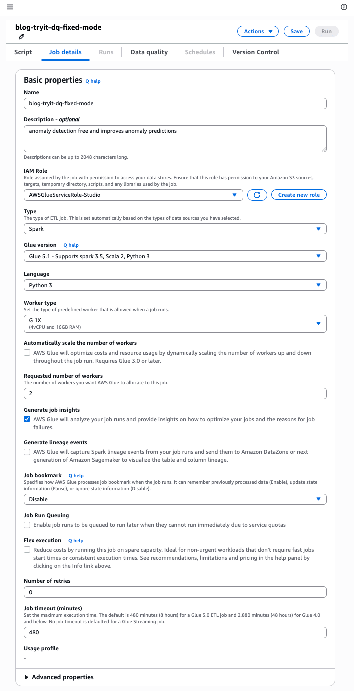
| Setting item | Value |
|---|---|
| Name | blog-tryit-dq-fixed-mode |
| IAM Role | AWSGlueServiceRole-Studio (Glue service role with S3 read permissions) |
| Glue version | Glue 5.1 |
| Language | Python 3 |
| Worker type | G.1X |
| Requested number of workers | 2 |
| Job timeout (minutes) | 10 |
Expand "Advanced properties" in the same "Job details" tab and add the input path parameter to "Job parameters."
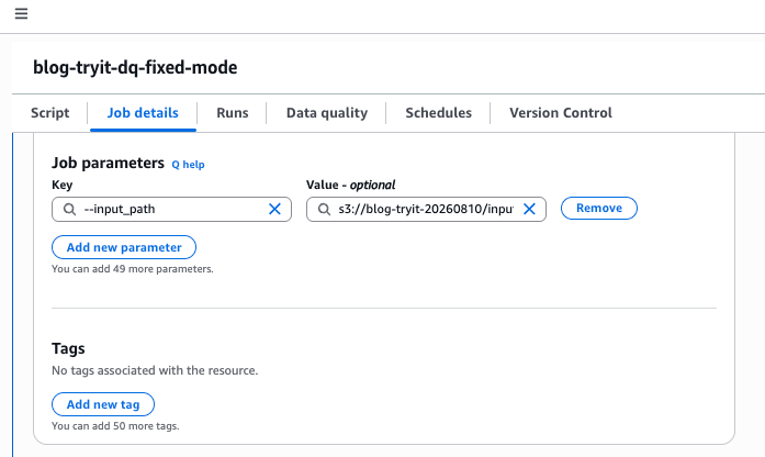
| Key | Value |
|---|---|
| --input_path | s3://blog-tryit-20260810/input/gen1/ |
Once configured, save the job using "Save" at the top right of the screen.
Running 5 Times While Swapping Data
Click "Run" at the top right of the screen to execute the job. Switch to the "Runs" tab and the running run will be displayed. Wait for the Run status to become "Succeeded."
Once the first run is complete, go back to the "Job details" tab, change the value of --input_path in Job parameters to s3://blog-tryit-20260810/input/gen2/, click "Save," and then click "Run" again. Repeat this through gen5 for a total of 5 executions.
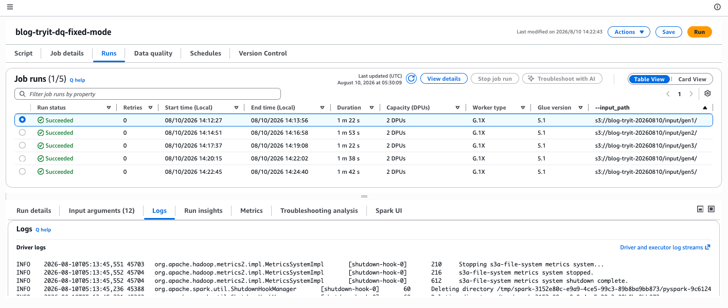
The results of the 5 runs can be listed in the "Runs" tab. The results this time are as follows, with all runs succeeding.
| Run | Input path | Row count | Run status | Execution time | DPU seconds |
|---|---|---|---|---|---|
| 1st run | input/gen1/ | 100 | Succeeded | 82 seconds | 164 |
| 2nd run | input/gen2/ | 102 | Succeeded | 113 seconds | 226 |
| 3rd run | input/gen3/ | 97 | Succeeded | 82 seconds | 164 |
| 4th run | input/gen4/ | 101 | Succeeded | 98 seconds | 197 |
| 5th run | input/gen5/ | 30 | Succeeded | 102 seconds | 204 |
Confirming Anomaly Detection Results
Open the "Data quality" tab of the job to display the data quality results for the selected run. You can switch the run to view using "Selected run" at the top right of the screen. Here, I selected the 5th run (30 rows).
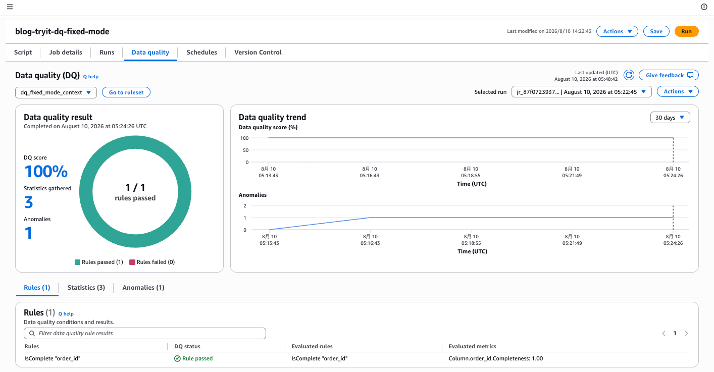
The summary is as follows.
| Item | Value |
|---|---|
| DQ score | 100% |
| rules passed | 1 / 1 |
| Statistics gathered | 3 |
| Anomalies | 1 |
The rule IsComplete "order_id" shows "Rule passed," and the evaluation metric was Column.order_id.Completeness: 1.00. While 1 anomaly was detected, the DQ score remains 100%. As stated in the official documentation, generating anomalies does not affect the data quality score.
At the bottom of the screen, there are 3 tabs: "Rules (1)," "Statistics (3)," and "Anomalies (1)." Let's look at Statistics and Anomalies in order.
Confirming Statistical Trends in the Statistics Tab
Selecting RowCount in the "Statistics" tab displays a graph of the collected statistics values over time. In addition to actual values (RowCount values), the model-calculated prediction trend (Prediction trend) and upper and lower bounds of the prediction (Prediction upper bound / Prediction lower bound) are overlaid.
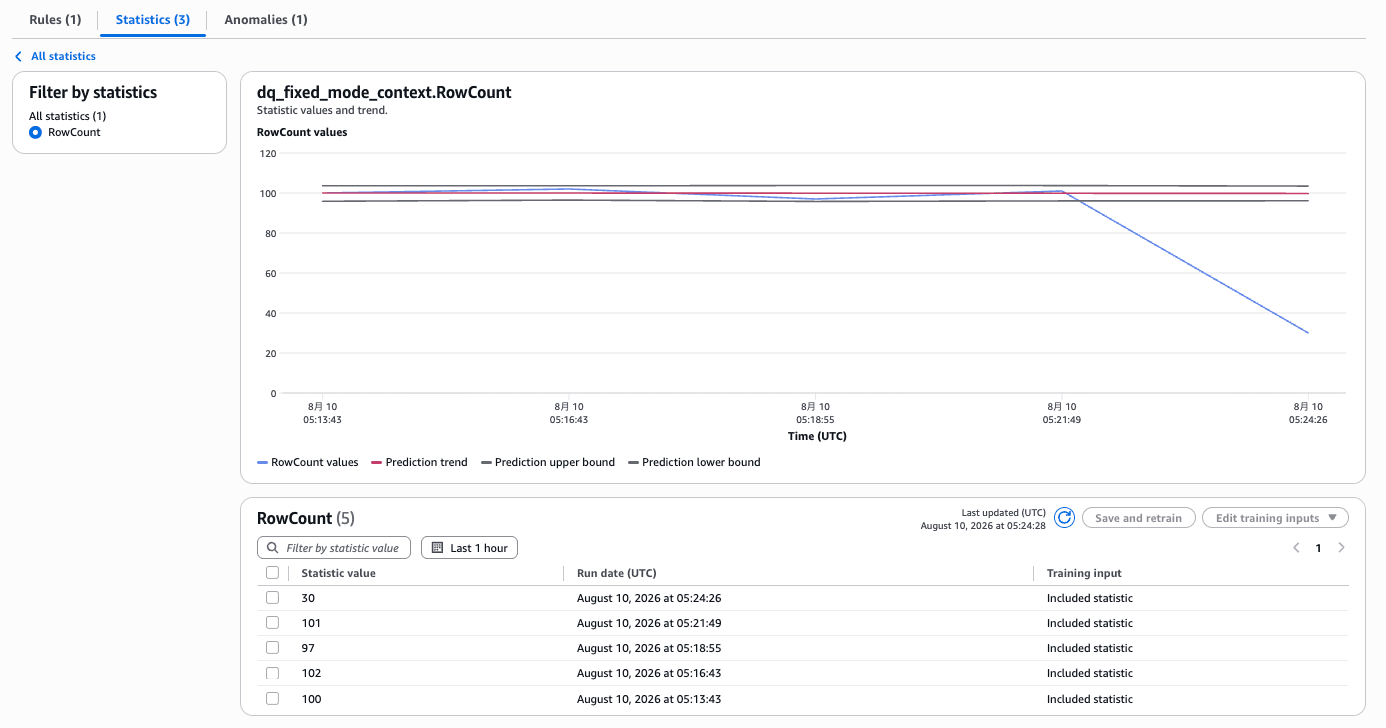
The recorded statistics values are as follows. All 5 runs are included as training inputs (Included statistic).
| Statistic value | Run date (UTC) | Training input |
|---|---|---|
| 30 | August 10, 2026 at 05:24:26 | Included statistic |
| 101 | August 10, 2026 at 05:21:49 | Included statistic |
| 97 | August 10, 2026 at 05:18:55 | Included statistic |
| 102 | August 10, 2026 at 05:16:43 | Included statistic |
| 100 | August 10, 2026 at 05:13:43 | Included statistic |
The prediction trend and upper/lower bound bands remain nearly horizontal around 100, and you can confirm from the graph the behavior of FIXED mode, which does not extrapolate linear trends. Only the last point (30) falls significantly below the lower bound.
Confirming Anomaly Details in the Anomalies Tab
The "Anomalies" tab lists the Observations generated in the currently selected run.
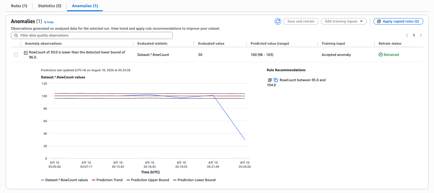
The detected anomaly was the following 1 item.
| Item | Value |
|---|---|
| Anomaly observations | RowCount of 30.0 is lower than the detected lower bound of 96.0. |
| Evaluated statistic | Dataset.*.RowCount |
| Evaluated value | 30 |
| Predicted value (range) | 100 (96 - 103) |
| Training input | Accepted anomaly |
| Retrain status | Retrained |
As expected, the sudden drop to 30 rows was detected as an anomaly. The predicted value is 100, the prediction range is 96 to 103, and the actual value of 30 falls well below the lower bound.
On the right side, "Rule Recommendations" presents recommended rules for detecting this anomaly as a rule in the future.
RowCount between 95.0 and 104.0
From "Apply copied rules," you can incorporate the recommended rules directly into the ruleset. You can also exclude specific statistical values from the training inputs using "Edit training inputs" and retrain the model with "Save and retrain." In this anomaly, Training input shows "Accepted anomaly" and Retrain status shows "Retrained," indicating the model was retrained with the detected value of 30 included in the training inputs. If you want to treat it as a true anomaly, edit the training inputs from here and retrain.
Confirming FIXED Mode Predictions (Constant Baseline)
From the results so far, let me organize how the FIXED mode predictions behaved.
The row count of the input data varied up and down at 100 → 102 → 97 → 101, but the prediction trend (Prediction trend) in the Statistics tab graph remained nearly horizontal. Even at the time of the 5th run when the anomaly was detected, the predicted value is 100 and the prediction range is 96 to 103. You can confirm the behavior of FIXED mode, which predicts near the mean of observed values as a constant baseline without extrapolating recent increases or decreases into the future.
Also, looking at the Run date of the statistics for the 5 runs in this verification, the execution intervals varied.
| Run | Run date (UTC) | Interval from previous run |
|---|---|---|
| 1st run | 05:13:43 | - |
| 2nd run | 05:16:43 | 3 minutes 00 seconds |
| 3rd run | 05:18:55 | 2 minutes 12 seconds |
| 4th run | 05:21:49 | 2 minutes 54 seconds |
| 5th run | 05:24:26 | 2 minutes 37 seconds |
Since FIXED mode treats all data points as equally spaced regardless of execution intervals, predictions are not pulled even when intervals are irregular like this. The prediction range remained stable and narrow at 96 to 103, allowing the sudden drop to 30 rows to be clearly detected as falling below the lower bound.
According to the official documentation, LINEAR mode learns trends and seasonality and extrapolates future values. For data without trends like this time, workloads with non-fixed execution intervals, and exploratory executions in notebooks, FIXED mode is said to be more suitable.
Discussion
Let me organize the knowledge gained from actually trying this out.
- The predicted values in FIXED mode are nearly constant (constant baseline), and even for data where row counts randomly increase and decrease, a prediction range with little noise was obtained. It is easy to use even for non-fixed-interval execution such as non-daily batch runs
- Since anomaly detection requires a minimum of 3 data points, the 1st through 3rd runs essentially serve as baseline building for learning. Since the prediction range is unstable while there are few data points, it seems good to run a few passes of data before going into production use
- Detected anomaly values are, as they are, learned by the model as normal values. This time as well, Training input showed "Accepted anomaly." If you want to treat it as a true anomaly, you need to exclude it from training inputs using "Edit training inputs" in the Anomalies tab and retrain with "Save and retrain"
- The job executions in this verification totaled 955 DPU seconds (approximately 0.27 DPU-hours) across 5 runs. Previously, in addition to this, an additional charge of 1 DPU per anomaly detection statistic was incurred, but with this update, anomaly detection in ETL jobs has no additional charge, making it easy to enable
Since specifying the observation mode is currently done via additional_options in the script, I would also like to see future improvements such as the ability to switch observation modes from the AWS Glue Studio visual editor and automatic recommendations for mode selection.
In Closing
AWS Glue Data Quality ETL anomaly detection is now available at no additional charge, and together with the new FIXED mode, I was able to confirm the behavior from the management console. Being able to detect a typical data quality problem—a sudden drop in row count—without setting thresholds and automatically generating recommended rules is practical.
For those who have previously held off on introducing anomaly detection due to cost concerns, why not try it out by adding analyzers to the EvaluateDataQuality of your existing Glue pipelines? I hope this article is useful to someone.