I tried anomaly detection for industrial sensors with SKAB and time series foundation models

Hello, I'm Morishige from Classmethod's Manufacturing Business Technology Division.

In the previous article Comparing Time Series Foundation Models Running on DGX Spark, I compared Chronos-2 and TimesFM 2.5 on prediction accuracy, latency, and context scaling using the ETTh1 benchmark. Near the end of that article, I briefly touched on the question "would anomaly detection work if we applied time series foundation models to PLC data in manufacturing?" in just one paragraph — my motivation this time is to dig deeper into that question with real data.

https://dev.classmethod.jp/articles/dgx-spark-timeseries-fm-3-bench/

I chose SKAB (Skoltech Anomaly Benchmark) as the subject. It contains 8-sensor time series recorded on an industrial pump testbed, with manually labeled real anomaly intervals. In the previous anomaly detection simulation I was artificially injecting Spike / Level shift / Noise burst patterns, but this time I observe how the models respond to anomaly patterns originating from real equipment.

The validation ran Chronos-2 (28M / 120M) and TimesFM 2.5 (200M) on DGX Spark and collected ROC AUC / F1 / FAR / MAR across all 34 datasets.

Overview of the SKAB Dataset

SKAB is an open dataset published on GitHub by Skoltech (Skolkovo Institute of Science and Technology). The license is GPL-3.0, and the data structure is as follows.

• 34 labeled CSV files (valve1/ 16 files, valve2/ 4 files, other/ 14 files) + 1 anomaly-free.csv
• Each CSV is sampled at 1 Hz with approximately 1,000 rows (about 16 minutes), totaling 37,401 rows
• 8 sensor columns (vibration acceleration ×2, current, voltage, pressure, body temperature, fluid temperature, flow rate) + anomaly label + changepoint marker
• Overall anomaly rate is 34.9%, with 129 changepoints

For reference, looking at the 8-sensor time series for valve1/0.csv, it looks like this. The red bands are the labeled anomaly intervals.

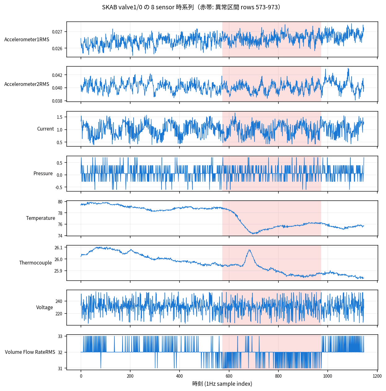
You can see that Voltage is on a ~230V scale and the Accelerometer is on a ~0.03 scale, with about 4 orders of magnitude difference between sensors. As I'll touch on later, how you absorb this scale difference is directly tied to anomaly detection accuracy.

In the anomaly interval (rows 573-974), Temperature and Thermocouple gradually rise, Volume Flow Rate fluctuates in small increments, and Voltage remains nearly normal. "Complex behavioral changes that are hard to notice from a single sensor alone" is a frequently seen pattern in SKAB anomalies.

Validation Approach

The anomaly detection flow was structured as follows.

1. Learn per-sensor z-score scalers from the anomaly-free section (the leading interval where anomaly=0 is continuous) of each dataset
2. Extract context and horizon windows with sliding_windows(context_len=256, horizon=16, stride=16), and assign the ground truth label for each horizon as "1 if at least one anomaly exists in the interval"
3. Generate predictions for the horizon interval with each model and compute per-sensor residuals in z-score space
4. Aggregate per-sensor residuals into a single anomaly score using one of mean / max / pca
5. Evaluate ranking capability with ROC AUC, and compute F1 / FAR / MAR using the best-F1 threshold

The reason for listing 4 evaluation metrics is that in manufacturing anomaly detection, the balance between miss rate (MAR) and false alarm rate (FAR) is the operational crux. F1 combines both into a single value, and ROC AUC is a threshold-independent ranking performance metric, making them easy to interpret.

Z-score normalization was added to absorb Voltage dominance. If you aggregate raw MSE, the MSE for Voltage alone is on the order of ~100 while other sensors are on the order of ~0.01, causing anomalies in other sensors to become invisible when dragged by just the one Voltage sensor. By standardizing per sensor, residuals from every sensor can be discussed on the same scale.

To ensure reproducibility of the validation, np.random.seed(0) and torch.manual_seed(0) were fixed, and each cell was run twice independently to obtain the standard deviation of AUC. The design adds a third run for datasets where the threshold exceeds 0.05. As a result, across all 4 cells × 34 datasets, there were 0 cases with std > 0.05, and both Chronos-2 and TimesFM 2.5 produced very stable results.

Validation Pipeline Overview

The full flow from data ingestion through aggregation and evaluation looks like this on one diagram.

Anomaly Detection with Chronos-2

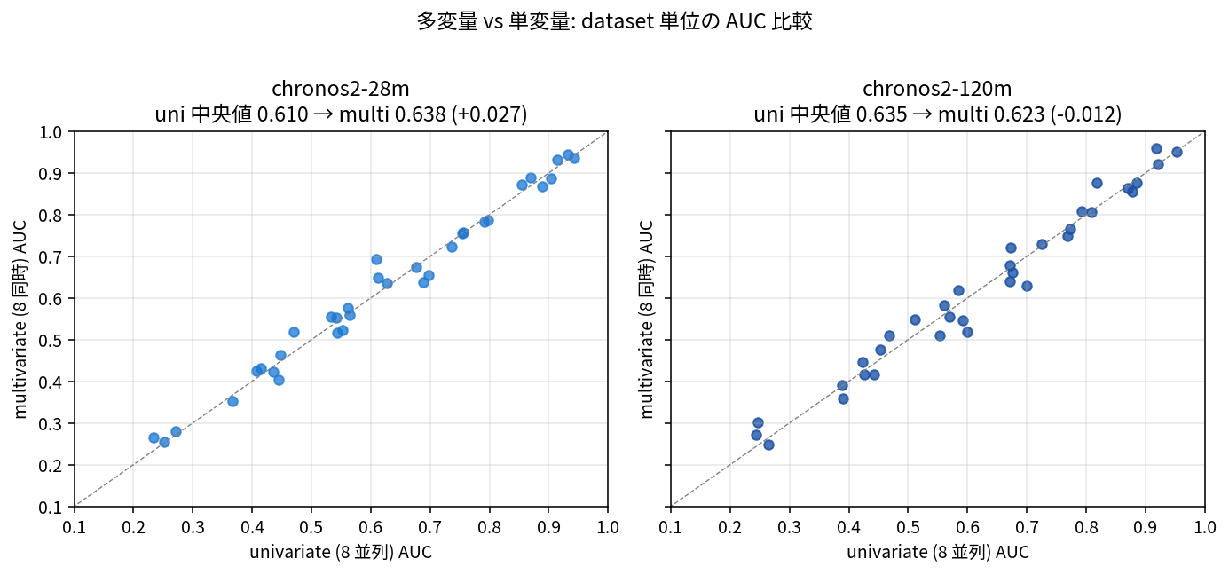
Chronos-2 (from AWS) returns predictions for multiple sensors at once in the form pipeline.predict_quantiles((1, n_var, ctx)). I collected latency and accuracy across all 34 datasets for both "multivariate mode" (feeding all 8 sensors together) and "univariate 8-parallel mode" (feeding 1 sensor at a time, 8 times).

Model × Mode	AUC Median	min	max	Warm Latency	GPU Memory
28M univariate	0.6103	0.234	0.942	3.7 ms / sensor	86 MB
28M multivariate	0.6376	0.255	0.945	4.1 ms / 8 sensor	88 MB
120M univariate	0.6351	0.244	0.952	6.5 ms / sensor	260 MB
120M multivariate	0.6234	0.247	0.960	7.3 ms / 8 sensor	264 MB

What stands out when looking at these numbers is that enabling multivariate for 28M raises AUC by +2.7 points, while for 120M it causes a slight regression of -1.2 points. In the previous ETTh1 benchmark, "120M multivariate showed a -7% improvement in OT MASE," so the trend is consistent — the picture that emerges is that 120M with ample capacity is sufficient in univariate mode, while the smaller 28M gets a boost from cross-channel attention.

The latency side is even clearer. When processing 8 sensors per window, 28M drops from 30 ms (8 univariate in parallel) to 4.1 ms in multivariate mode, and 120M drops from 52 ms to 7.3 ms — roughly a 7× speedup for both. Since one forward pass returns predictions for all 8 sensors, multivariate mode is not just cost-free but actually a net positive.

Against a PLC scan cycle budget (typically 100 ms to 1 second), Chronos-2 28M multivariate at 4.1 ms has more than 25× headroom. GPU memory is also around 88 MB, a size that comfortably fits on edge devices like the Jetson Orin Nano class. Among the 34 datasets, 28M multivariate outperformed 120M multivariate in 18 of them, so there is little reason to discard 28M when edge deployment is in scope.

Anomaly Detection with TimesFM 2.5

TimesFM 2.5's forecast(inputs=[1Darray]) is a univariate-only API that takes a list of 1D inputs. To handle multivariate data, you independently predict 8 sensors and then aggregate the residuals into one score in the downstream step. I compared three aggregation strategies: mean / max / pca.

Aggregation	AUC Median	min	max	Best suited for
mean	0.7723	0.328	0.898	Situations where all sensors show anomalies equally
max	0.6923	0.364	0.830	Situations dominated by sudden spikes in a single sensor
pca	0.5538	0.216	0.875	Situations where periodic correlation structure breaks (theoretically)

Looking at the numbers, mean pulls ahead of the others by a margin, with a median of 0.77. While max is good at catching sudden spikes in a single sensor, its weakness of being sensitive to noise showed up here. PCA in theory aims for "anomalies that deviate from the normal correlation structure," but with SKAB's dataset size (roughly 30-60 windows per dataset), the estimation of the first principal component tends to be unstable, resulting in AUC even lower than max.

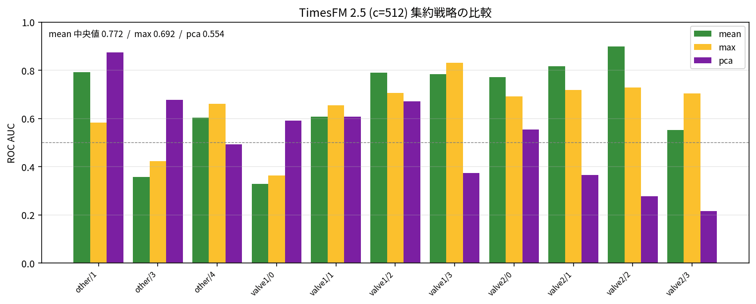
However, looking at per-dataset distributions, in other/1 pca tops all three strategies at 0.875, and in other/3 it holds its own at 0.678. It's the classic case-by-case situation common in manufacturing anomaly detection — mean wins on average, but other strategies land better in specific cases.

The next thing to examine is context scaling — how far back to look. SKAB's datasets are about 1,000 rows each (roughly 16 minutes). I ran TimesFM 2.5 with contexts of 128 (about 2 minutes) and 512 (about 8 minutes) and compared them. In the parent article, extending to c=15,360 improved MASE by 30%, so I expected "longer context should always be better for anomaly detection too" — but as it turned out, it wasn't that simple.

Context	AUC Median (mean agg.)	std	Evaluable datasets
c=128	0.6822	0.162	12
c=512	0.7723	0.182	11

Overall, c=512 wins by about +0.06, but at the per-dataset level, some pairs reverse.

Dataset	c=128	c=512	Δ	Interpretation
valve1/0	0.5426	0.3284	-0.214	Short context is better
valve2/3	0.7324	0.5520	-0.180	Short context is better
other/1	0.4231	0.7917	+0.369	Long context is essential
valve1/2	0.6523	0.7902	+0.138	Long context is better

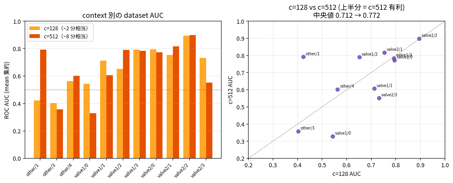
Translated into manufacturing terms: short context is suited for instantaneous anomalies like sudden valve blockages or sharp shifts. On the other hand, long-term trend anomalies like disruptions to operating cycles or breakdown of periodicity require long context — with c=128, they are dismissed as "normal for this equipment." Running short-context and long-context models in parallel and combining both anomaly scores as an ensemble is a natural option that comes to mind.

I also tried c=2048, but even the longest SKAB dataset has only 1,328 rows, failing to meet the context + horizon ≤ T constraint, making all datasets unevaluable. Within the SKAB scale, comparing c=128 and c=512 is the practical range.

How to Use Each of the 3 Models

Having looked at Chronos-2 and TimesFM 2.5 individually, let me now line them up side by side on the same 11-dataset subset. Since the TimesFM side was sampled at 12 datasets for inference cost reasons (other/2 was excluded because no positive labels appeared), I re-computed the AUC median for Chronos-2 as well, limited to these 11 datasets.

Cell	AUC Median	std	min	max	Warm Latency	GPU Memory
chronos2-28m univariate	0.5648	0.196	0.251	0.942	3.7 ms / sensor	86 MB
chronos2-28m multivariate	0.5602	0.191	0.255	0.937	4.1 ms / 8 sensor	88 MB
chronos2-120m univariate	0.5926	0.192	0.244	0.921	6.5 ms / sensor	260 MB
chronos2-120m multivariate	0.5557	0.189	0.272	0.921	7.3 ms / 8 sensor	264 MB
TimesFM 2.5 mean (c=512)	0.7723	0.182	0.328	0.898	229 ms / sensor	944 MB
TimesFM 2.5 max (c=512)	0.6923	0.131	0.364	0.830	Same as above	Same above

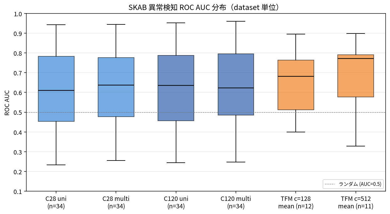
TimesFM 2.5 mean outperforms all Chronos-2 variants by +18 to +22 AUC points (in relative terms, +30 to +39%). However, tracking per-dataset results reveals that the two models capture anomalies quite differently.

Dataset	C28 multi	C120 multi	TFM mean	Pattern
valve2/1	0.43	0.42	0.82	Hard cases that TimesFM catches
valve2/3	0.26	0.27	0.55	Same as above
valve1/0	0.52	0.56	0.33	Only Chronos-2 catches it
other/4	0.79	0.81	0.60	Same as above
valve2/2	0.94	0.92	0.90	Both models perform well

Roughly summarizing: TimesFM nearly doubles the AUC on hard cases where Chronos-2 completely fails (valve2/1, valve2/3), while Chronos-2 maintains middle-tier or better scores on valve1/0 and other/4 where TimesFM drops. This is consistent with the hypothesis that "long-term trend anomalies favor TimesFM, short-term spike anomalies favor Chronos-2," and points toward an ensemble of both models as the next logical step.

On the latency side, the picture looks very different.

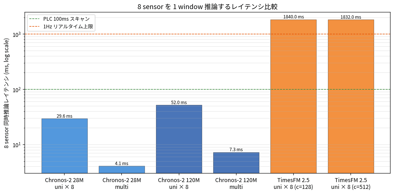
The gap between Chronos-2 28M multivariate (4.1 ms) and TimesFM 2.5 (approximately 1,832 ms) is about 450×. TimesFM wins on accuracy, but it doesn't fit within the PLC scan cycle budget of 100 ms, and doesn't even make the 1 Hz real-time judgment ceiling of 1,000 ms.

The practical guidance for choosing between them looks something like this.

Scenario	Recommendation
Edge deployment (PLC-direct IPC, Jetson, etc.) + real-time judgment	Chronos-2 28M multivariate (4 ms / 88 MB)
Factory server (aggregating multiple lines) + medium accuracy	Chronos-2 120M (uni or multi)
Server aggregation + accuracy-first (batch judgment OK)	TimesFM 2.5 mean (c=512) (229 ms / 944 MB)
Don't want to miss either anomaly type	Ensemble of Chronos-2 28M multi + TimesFM 2.5 mean

In manufacturing facilities, the standard approach is two-stage judgment — first-pass triage at the edge, then re-evaluation on the server for anything suspicious — so a setup placing Chronos-2 28M at the edge and TimesFM 2.5 at the aggregation layer seems like the natural landing point.

Detection Example

Numbers alone can be hard to visualize, so let me walk through how Chronos-2 28M multivariate detects anomalies specifically on valve1/4 (a dataset with AUC 0.87).

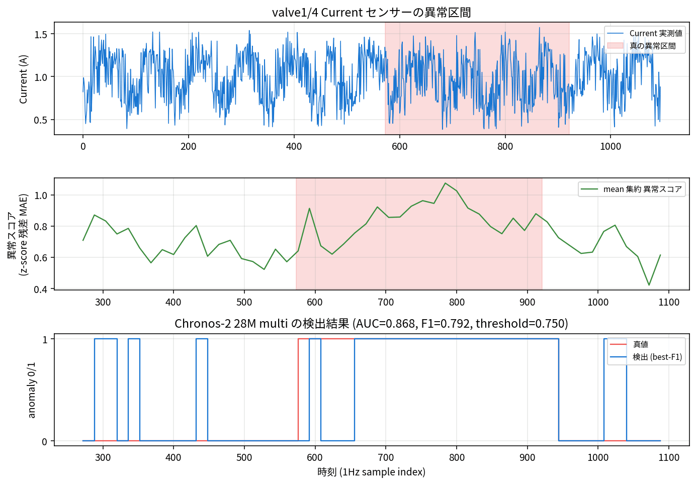
The top panel shows the raw Current sensor signal (red band is the true anomaly interval), the middle panel shows the per-window anomaly score aggregated with mean, and the bottom panel overlays the 0/1 detection result at the best-F1 threshold against the ground truth. The result of AUC 0.868 / F1 0.792 / threshold 0.750 is not bad for manufacturing anomaly detection.

Worth noting is that while the anomaly score clearly peaks in the true anomaly interval (around rows 600 to 950), several small peaks around 0.5 also appear during the preceding normal interval. In practice, it is hard to suppress false positives to zero in noisy normal states, and even with threshold optimization using best-F1, the result is FAR of 3.4% and MAR of 30.4%. If you want to err on the safe side, you need to lower the threshold to increase FAR and suppress MAR — that trade-off is the key discussion point when taking this from PoC to production.

How to Set Up PLC Real-Time Integration

As a way to replicate the "PLC → time series model" loop without actual PLC hardware, OpenPLC (an open-source PLC emulator) combined with Node-RED is an option. A setup that streams SKAB CSV over Modbus TCP and returns anomaly scores from Chronos-2 looks like this.

The latency budget breaks down as: PLC scan (1 Hz, 1,000 ms) → InfluxDB write + latest window retrieval (5-20 ms) → Chronos-2 28M multivariate inference (4 ms) → threshold judgment + notification (1-5 ms), with the entire inference pipeline completing in 10-30 ms. Even if the scan cycle rises to 100 ms, Chronos-2 28M handles it fine; TimesFM 2.5 at 1,832 ms would not make it.

In terms of implementation, keeping a deque on the Node-RED side instead of fetching 256 rows from InfluxDB each time yields lower latency; the z-score scaler learned from the anomaly-free section should be saved in advance and applied only at inference time; and Chronos-2's multivariate input expects a 3D tensor of shape (1, n_var, ctx) — covering these three points will let you operate close to the 4 ms latency measured in this article.

3-Tier Architecture Combined with SCADA / MES

In actual manufacturing facilities, PLC is layered under SCADA, which is layered under MES, and which tier to place the time series foundation model in depends on line scale. For small scale: edge inference directly connected to PLC. For medium scale: SCADA aggregates data and passes it to the model, which returns anomaly scores to the HMI. For large scale: multivariate prediction combining SCADA tags and MES process instructions is fed back to MES for quality traceability at the process lot level. The three-tier model selection guidance maps naturally onto this hierarchy.

The roles divide cleanly: L1 for immediate alerts, L2 for detailed evaluation via two-model ensemble, and L3 for daily and lot-level roll-up analysis. The Cognite × NVIDIA × Celanese case study introduced in Chapter 7 of the parent article can also be read as a setup where NV-Tesseract plays an active role at L2/L3, so reading it alongside this article's Chronos-2 / TimesFM 2.5 results should give you a clearer picture of the manufacturing AI stack as a whole.

Summary

Evaluating whether Chronos-2 and TimesFM 2.5 "can be used" and "how to use them differently" against SKAB anomaly data derived from real equipment across all 34 datasets revealed roughly the following points.

• Going multivariate is not just cost-free — it's a gain. Enabling multivariate for Chronos-2 28M raises AUC by +2.7 points and speeds up latency by about 7×.
• Models have clearly different strengths by anomaly type. TimesFM 2.5 mean leads overall with a median AUC of 0.77, yet in datasets where Chronos-2 excels (such as valve1/0), TimesFM falls off — a complementary relationship.
• Context scaling is not "longer is always better" — switching TimesFM 2.5 between c=128 and c=512 produces reversals of ±0.37 depending on the dataset.
• Balancing PLC scan cycle budget against accuracy requirements, a 3-tier setup of edge 28M / server 120M + TimesFM is the realistic solution, and Chronos-2 28M multivariate (4 ms / 88 MB) can be used as-is for the edge tier.

Once NV-Tesseract (currently at evaluation license stage) becomes available to run locally, I'd like to revisit a comparison against TimesFM 2.5 at the L2/L3 tiers. Reading the Cognite × NVIDIA × Celanese case study's 4-sensor state prediction alongside this article's 8-sensor anomaly detection should help paint a picture of the manufacturing AI stack for 2026.

Reference Links

• SKAB (Skoltech Anomaly Benchmark)
• Chronos-2 (amazon/chronos-2)
• Chronos-2 Small (autogluon/chronos-2-small)
• TimesFM 2.5 (google/timesfm-2.5-200m-pytorch)
• OpenPLC Runtime
• Node-RED
• Previous article: Comparing Time Series Foundation Models Running on DGX Spark