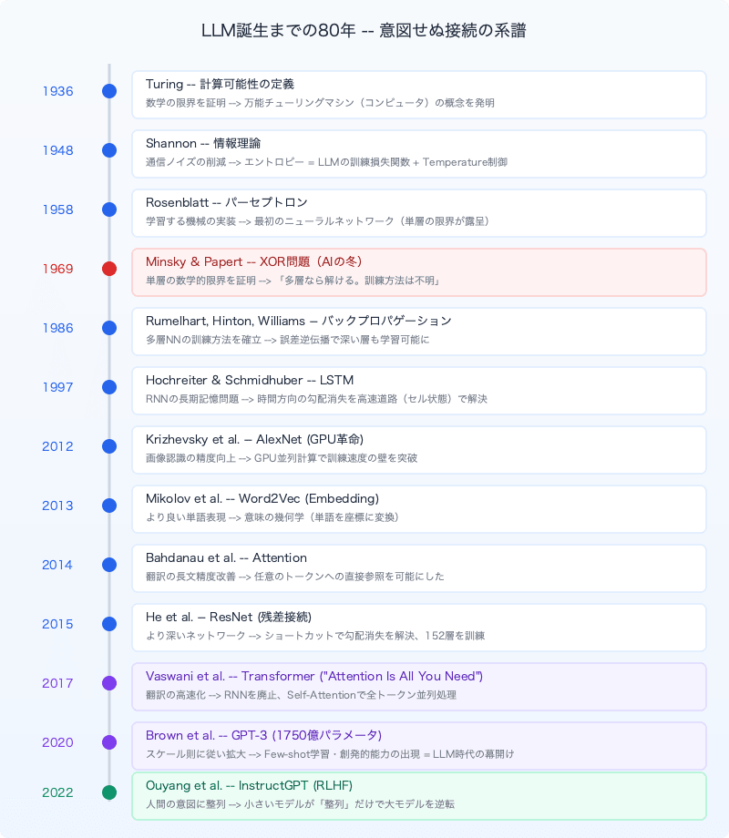
"The Accumulation of Failures" Gave Birth to LLMs (Part 2) — From Attention to the Scaling Revolution, and Then to Alignment
This page has been translated by machine translation. View original
Introduction
This article is a continuation of Part 1.
In Part 1, we traced the journey from Turing machines to Shannon's information theory, perceptrons and backpropagation, the acceleration of training with GPUs and overcoming vanishing gradients, and the Word2Vec/Embedding technology that "converts words into meaningful vectors."
In Part 2, we start from the question of how to handle context, and follow the second half of the story of how LLMs came to be "without being designed" — through the structural limitations of RNNs, the birth of Attention, the evolution into Transformer, the scale revolution of GPT-3, and the present era of alignment and efficiency through RLHF.
Chapter 5 — How Do We Handle Context? — The Birth of Attention
Note: The research on LSTM (1997) and RNNs themselves that appears in this chapter chronologically predates AlexNet (2012) and Word2Vec (2013). However, understanding "why ordered data is difficult" requires the knowledge from Chapter 3 (training neural networks and the wall of depth) and Chapter 4 (how to convert words into vectors) as prerequisites, which is why they are covered in this order.
Why Machine Translation Was the Main Battlefield
In the early 2010s, the application field that NLP (Natural Language Processing) researchers were putting the most effort into was machine translation.
The reason is simple. Translation is the task that most rigorously tests "whether language is truly being understood." You cannot translate by simply replacing words one by one. Word order changes, grammar changes, cultural nuances change. You need to understand the meaning of the entire sentence and reconstruct it in another language.
English:  The cat sat on the mat.
Japanese: 猫がマットの上に座った。

Word replacement only: The=その cat=猫 sat=座った on=の上に the=その mat=マット
→ 「その猫座ったの上にそのマット」 ← Meaningless

Correct translation requires restructuring word order, adding particles, removing articles
→ Premised on understanding the meaning of the entire sentence
So the limits of "how far machines can handle language" were exposed earliest in translation. And the technology born to resolve that bottleneck later became the foundation for all of LLMs.
The Bottleneck of Translation Models: Structural Limitations of RNNs (around 2014)
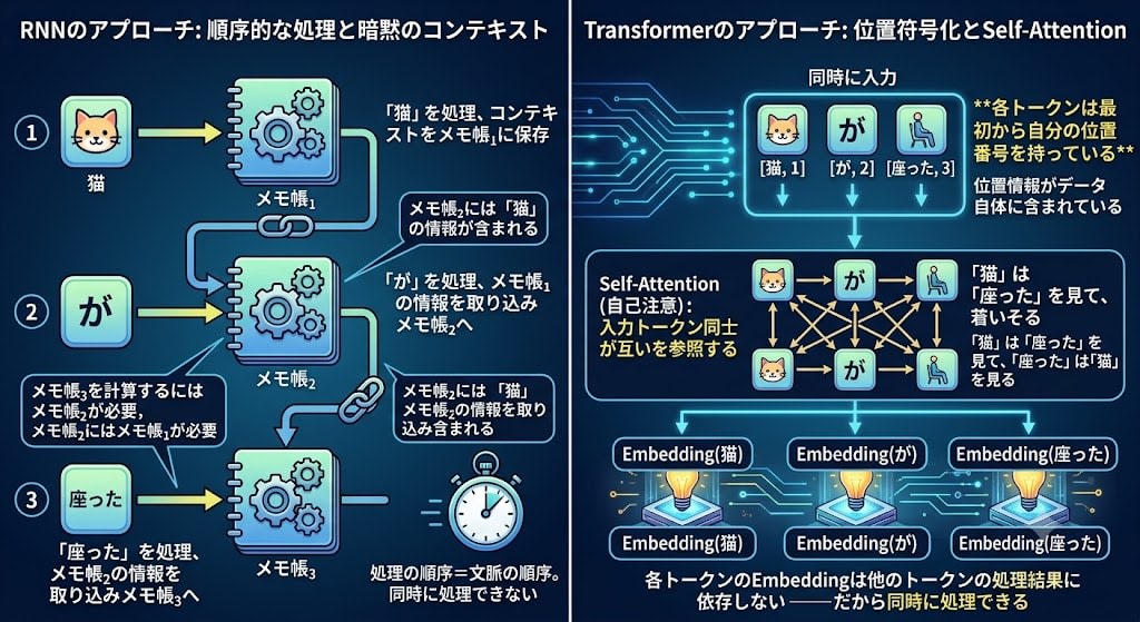
Translation models at the time used RNNs (Recurrent Neural Networks). RNNs were the best option available for handling context.
RNNs were not a new invention — they were a combination of the components we had seen so far. The internal neurons, weights, layers, and backpropagation are the same as in Chapter 3. What they receive as input are the Embedding vectors from Chapter 4. To understand RNN's single new idea, we first need to know the limitations of ordinary neural networks.
Up to this point, neural networks had succeeded with data that can be input all at once, like images. When AlexNet classifies a photo of a cat, one million pixels are fed simultaneously into the input layer. It doesn't process "first look at the top-left pixel, then look at the pixel to the right..." The entire image is input at once, so there's no need to "remember what came before."
However, language is fundamentally data arranged in order. The meaning of "The cat sat on the mat" depends on the order of the words. "The mat sat on the cat" has completely different meaning with the same words. And to understand the second half of a sentence, you need to remember what was said in the first half.
Image:    [all 1 million pixels] → input simultaneously → "photo of a cat"
          No order. No memory needed.

Language: "The" → "cat" → "sat" → "on" → "the" → "mat"
          Ordered. To understand "sat," you need to remember "The cat."
To put this in a familiar analogy, it's similar to taking notes while listening to a lecture.
- Ordinary network = Listens to the lecture but takes no notes. Forgets after each sentence. Can only respond to the sentence currently being heard.
- RNN (explained below) = Takes notes in a one-page notepad while listening to the lecture. When the notepad is full, overwrites old notes with new content. When the lecture ends, only that one page remains.
With this analogy in mind, let's look at the technical mechanism.
So what happens when we try to process a sentence with an ordinary neural network?
Attempting to process a sentence with an ordinary network (no note-taking):

  "The" → [input layer]→[hidden layer]→[output layer] → result 1    ← processing complete, network resets
  "cat" → [input layer]→[hidden layer]→[output layer] → result 2    ← zero trace of "The"
  "sat" → [input layer]→[hidden layer]→[output layer] → result 3    ← zero trace of "The cat"
You might think "since each layer receives the output of the previous layer, isn't information carried over?" But that refers to the flow of one input passing through multiple layers (a spatial flow). The flow of "The" through input layer → hidden layer → output layer is the process of a single word progressing to deeper layers.
The problem is temporal flow. When processing of "The" finishes and processing of "cat" begins, the network is completely reset. There's no trace of "The" left in the hidden layer. So when processing "sat," there's no way to know "what sat (the cat did)."
Spatial flow (one input passes through multiple layers) ← this exists even in ordinary networks
  "cat" → [Layer 1] → [Layer 2] → [Layer 3] → output

Temporal flow (multiple inputs are processed in order) ← this doesn't exist in ordinary networks
  time 1: "The" → process → complete → reset
  time 2: "cat" → process → complete → reset  ← doesn't remember "The"
  time 3: "sat" → process → complete → reset  ← doesn't remember "The cat"
RNN's Solution: The Same Layer Carries Memory Forward
The idea of RNNs is that the same layer processes tokens of different time steps in order, carrying its internal state (notepad) over to the next time step.
How the components combine:

Chapter 3 components:  neurons, weights, layers, backpropagation
                ↓ (used as the internal structure of RNN)
Chapter 4 components:  Embedding (word → vector conversion)
                ↓ (used as input to RNN)
Chapter 5's new element: the same layer carries the notepad across time steps
                ↓
              = RNN (a neural network that can process ordered data)
This "notepad" is technically called the hidden state. Do you remember "hidden layer" from Chapter 3 — the internal workspace between the input and output layers, invisible to the user? The RNN's "hidden state" is the same "hidden." It's called "hidden" because it's intermediate data inside the network that doesn't directly appear in either the input (the word currently being read) or the output (the translation result).
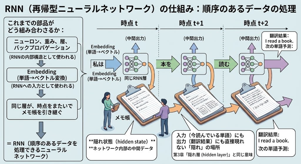
The key point is that in RNNs, the same hidden layer is used repeatedly (Recurrent = recursively). Rather than a relay of different layers, one layer operates repeatedly at each time step, and by carrying the notepad forward, it can remember "what it read before."
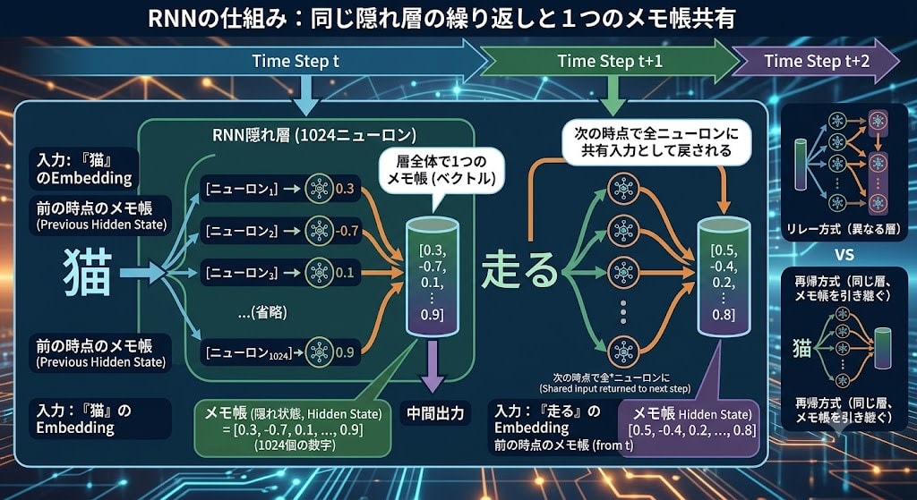
And the notepad is not held individually by each neuron — there is one per entire layer. If the hidden layer has 1,024 neurons, each neuron outputs one number, and those 1,024 numbers gathered together form the "notepad" vector. At the next time step, these 1,024 numbers are fed back as shared input to all neurons in the layer.
One time step of the hidden layer (1,024 neurons):

  Input: Embedding of "cat" + notepad from previous time step
          ↓
  [neuron₁] → 0.3   ─┐
  [neuron₂] → -0.7  ─┤
  [neuron₃] → 0.1   ─┼→ notepad = [0.3, -0.7, 0.1, ..., 0.9] (1,024 numbers)
  ...                  │
  [neuron₁₀₂₄] → 0.9 ┘
          ↓
  This notepad is shared to all neurons at the next time step
If you know React, it might help to think of the RNN's hidden state as similar to
useRef.ref.currentretains its value across renders, and updating it doesn't trigger a re-render — meaning it's an internal state "hidden" from React's system. The RNN's notepad works the same way:ref.currentis overwritten and updated with each time step (token processing), always holding only the latest state. Old values are overwritten and disappear.const memo = useRef(new Float32Array(1024)); function processToken(embedding) { memo.current = computeNewState(embedding, memo.current); // Old memo.current is overwritten and disappears } processToken(embed("cat")); // memo.current = [info about cat] processToken(embed("sat")); // memo.current = [info about cat sat...] processToken(embed("on")); // memo.current = [info about cat sat on...]
At each step, the RNN can only use two things — "the Embedding vector of the word currently being read" and "the notepad passed from the previous step." It cannot go back and re-read previous words. Information that has been read exists only within the notepad. In the lecture analogy, it's like writing continuously in a one-page notepad with no way to rewind the lecture.
Intuitively, it might seem more natural for each neuron to have its own dedicated notepad. But the reason the RNN's notepad is shared across the entire layer is that each neuron's output becomes context for other neurons.
When processing "The cat sat," suppose one neuron detects "the subject is cat" and another detects "the verb is past tense." When processing the next token, a compound understanding is needed — "the subject of the past-tense verb is cat." This cannot be held by a single neuron alone — it's information that can only be formed by combining the outputs of multiple neurons.
By sharing a notepad as a vector combining all neurons' outputs (1,024 numbers) and feeding it as input to all neurons at the next time step, each neuron can reference what other neurons detected at the previous time step. With independent notepads per neuron, this "horizontal information sharing" would be impossible.
How Neurons Use the Notepad
At each time step, each neuron receives as input a single vector — the concatenation of "the current token's Embedding" and "the notepad from the previous time step" — and performs the same multiplication and addition as in Chapter 3. The neuron itself doesn't know "which part is the token and which part is the notepad." But through training, the weights for the token and the weights for the notepad learn different roles. For example, a pattern like "if the current token is a verb, heavily weigh the information in the notepad corresponding to the subject" naturally emerges as weight values.
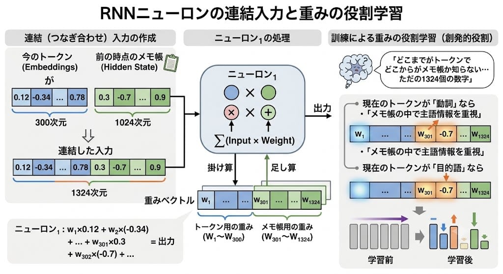
What pattern each neuron learns is not predetermined. Through the training process, each neuron finds on its own "some pattern useful for predicting the next token." That pattern may be an abstract one that humans cannot interpret. This is one of the reasons neural networks are called "black boxes."
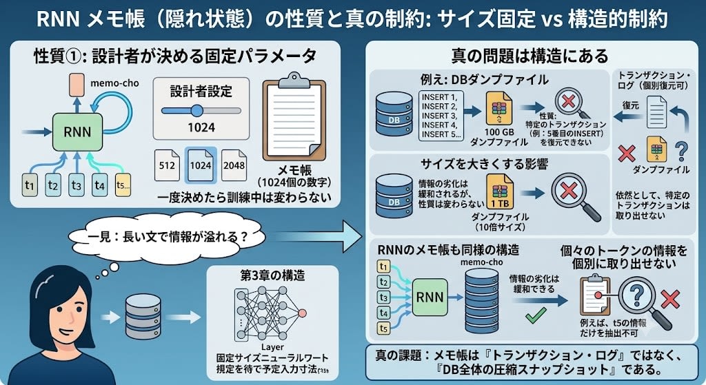
The Real Bottleneck of RNNs: You Can't Query a Snapshot
The size of the notepad (1,024 numbers) is a parameter that the designer decides before training. It could be 512 or 2,048, but once decided it doesn't change — this is because neural network layers expect a fixed number of inputs (recall the structure from Chapter 3).
"The size is fixed, so information overflows with long sentences" — this appears to be the problem at first glance. But the real problem is not size, it's the data structure.
The notepad is similar to a database snapshot (dump). A dump file reflects the cumulative result of all past transactions, but you cannot restore a specific INSERT statement. Even if you make the size 10 times or 1,000 times larger, this property doesn't change.
The RNN's notepad is the same. All past tokens have contributed to the current state, but the structural constraint that individual token information cannot be extracted individually doesn't change no matter how large you make the notepad.
In translation models, you read the entire input sentence before starting to generate the output sentence.
Input sentence → [RNN: reads one word at a time, updates notepad] → final notepad (snapshot) → [output RNN] → translated sentence
When the output RNN generates the translated sentence, all it has is the final snapshot. For example, when translating "She went to the market. There she met her friend's girlfriend" — when the output RNN translates the third "her/she," it would want to reference the corresponding part of the input sentence to confirm it refers to "the friend's girlfriend." But each token has dissolved into the snapshot. There's no way to extract it pinpoint.
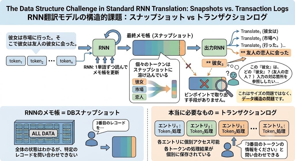
What's truly needed is not a snapshot but a transaction log — a data structure where the processing results of each token are saved individually and can be queried. This shift is the core of the Attention that appears later.
Déjà vu from Chapter 3: Vanishing Gradients, Again
RNN's problems weren't limited to information overflow. Learning itself also hit a wall.
In Chapter 3, we saw the mechanism of backpropagation (error backpropagation). Compare the output to the correct answer, propagate the error signal in reverse, and adjust the weights of each layer — a "blame" mechanism that tracks "how much each weight contributed to the mistake."
The same mechanism is used in RNNs. But in Chapter 3, error signals flowed backward across layers, while in RNNs they flow backward across time steps.
For example, when a prediction is wrong at the 50th token, "the way the 1st token was processed being wrong" might be the cause. But the error signal needs to trace back 49 times through the chain of notepads, and the signal shrinks at each step. As a result, feedback for early tokens approaches zero and weights aren't adjusted — meaning the network cannot learn "how to properly process the beginning of a sentence."
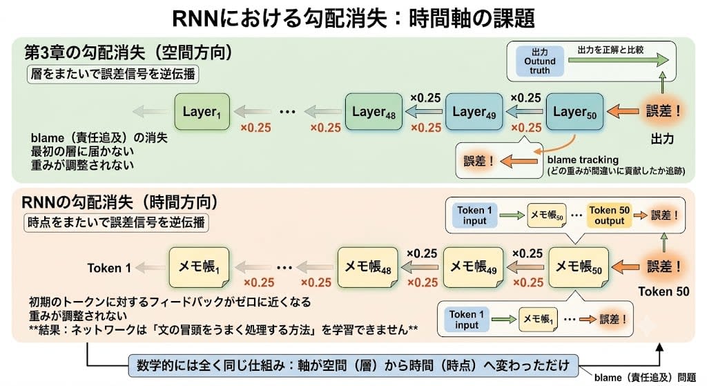
The math is exactly the same. In Chapter 3, signals disappeared as they passed through deep layers. In RNNs, signals disappear as they trace back through long time spans. Only the axis changed from space to time — the same problem appeared again.
LSTM: ResNet for the Time Direction (invented in 1997, became the mainstay of translation from 2014)
In Chapter 3, ResNet (residual connections) solved the vanishing gradient problem in the layer direction. It's a mechanism that adds the input to the output via a shortcut, creating a "highway" where gradients can flow directly.
Then what about vanishing gradients in the time direction? In fact, a solution based on the same idea was proposed 18 years before ResNet (2015) — in 1997. LSTM (Long Short-Term Memory) by Hochreiter and Schmidhuber. It remained a niche existence for many years, but around 2014 it flourished as the main architecture for machine translation, coinciding with the deep learning boom and the spread of GPUs.
The core of LSTM is having another memory called cell state in addition to the ordinary notepad. This cell state is a highway that passes through mostly unchanged between time steps.
LSTM also has a mechanism called gates. Three gates — "forget gate," "input gate," and "output gate" — control "what to forget," "what to write," and "what to read out" with respect to the cell state. This allows important information to be retained for long periods while discarding unnecessary information.
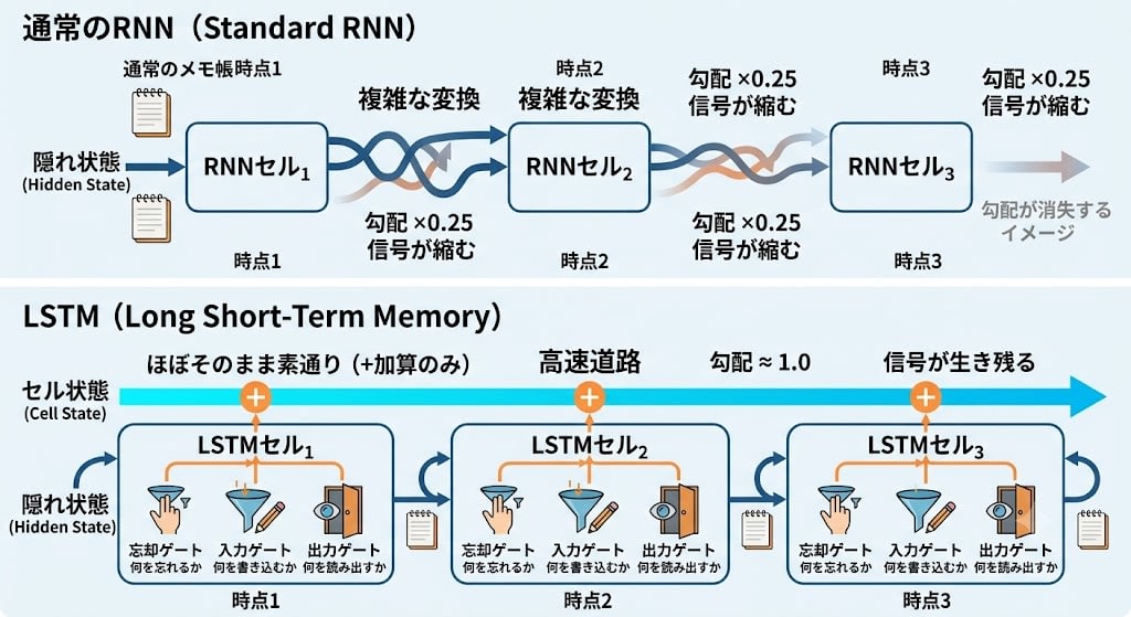
LSTM greatly improved the memory problem of RNNs and was used as the mainstay in machine translation around 2014–2017. However, a fundamental constraint remained — sequential processing. Process token 1, then token 2, then token 3 after token 2. No matter how much memory improved, the parallel computation of GPUs couldn't be utilized.
A Patch for the Bug: Attention
Bahdanau et al.'s solution was precisely the "from snapshot to transaction log" shift described earlier.
Step 1: Turn the Snapshot into a Transaction Log
When RNNs process input, they update the notepad (snapshot) at each step. Conventionally, only this final snapshot was passed to the output RNN. Bahdanau et al.'s idea was to save each step's snapshot as independent copies, all kept.
The important thing is that what's saved is not a delta (diff) but a complete snapshot at each time step. If 5 tokens are processed, 1,024 numbers × 5 sets — a total of 5,120 numbers are saved.
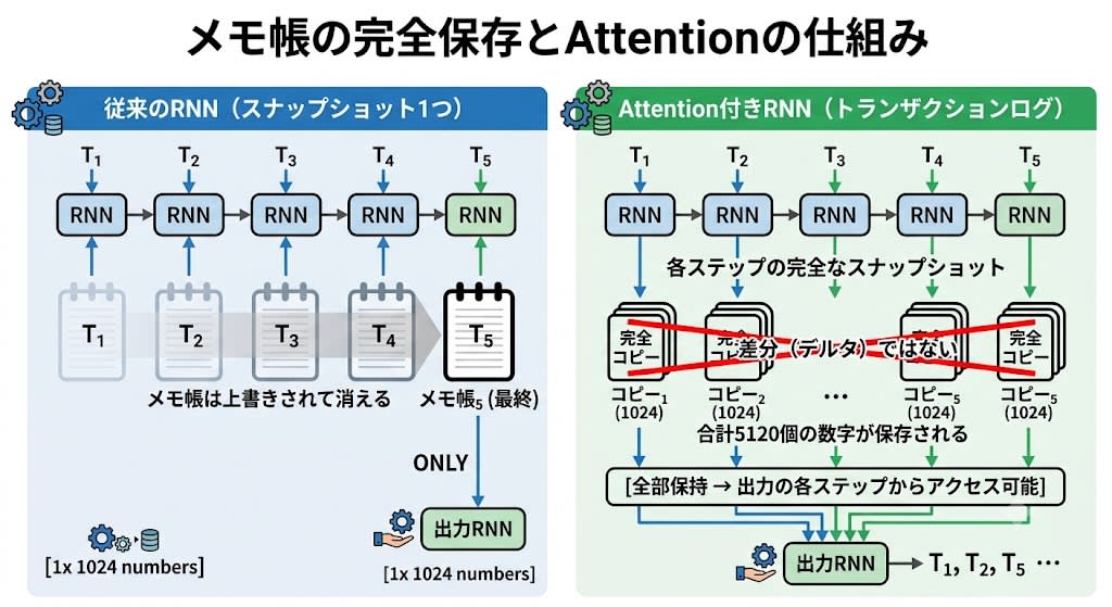
In React terms, Attention is like saving a spread copy with
history.push([...memo.current])before overwritingref.current. At output time, you can access the state at any point in time withhistory[i].
Returning to the lecture analogy, Attention corresponds to recording the lecture. Rather than relying only on notes (the final notepad), recordings of each point in the lecture remain.
But having recordings alone is not enough. You can't replay the entire 2-hour lecture recording every time. You need a mechanism to judge "which part should be replayed now." This is the core of Attention.
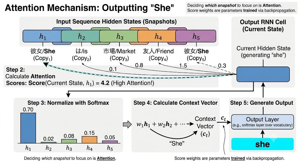
Step 2: Learning Which Snapshot to Focus On
When the output RNN generates each word of the translation, the following process runs:
- Take the current state of the output RNN ("what is currently being translated")
- Calculate relevance scores with each of all saved snapshots
- Normalize the scores with softmax to convert them into weights that sum to 1.0
- Take a weighted average of the snapshots according to the weights to create a context vector
- Use this context vector to generate the output word
These weights that determine "which snapshot to pay how much attention to" — this is the origin of the name Attention. When humans read text, they don't pay equal attention to every word, but focus attention on parts relevant to the current context. The Attention mechanism recreates exactly this numerically.
And the weights used in score calculation are also parameters trained by backpropagation. Patterns like "when translating a verb, give high scores to the snapshot for the subject" are automatically learned from data.
Attention Also Improves Vanishing Gradients
There is another important effect of Attention. The direct connections from the output to each snapshot become shortcuts for gradients.
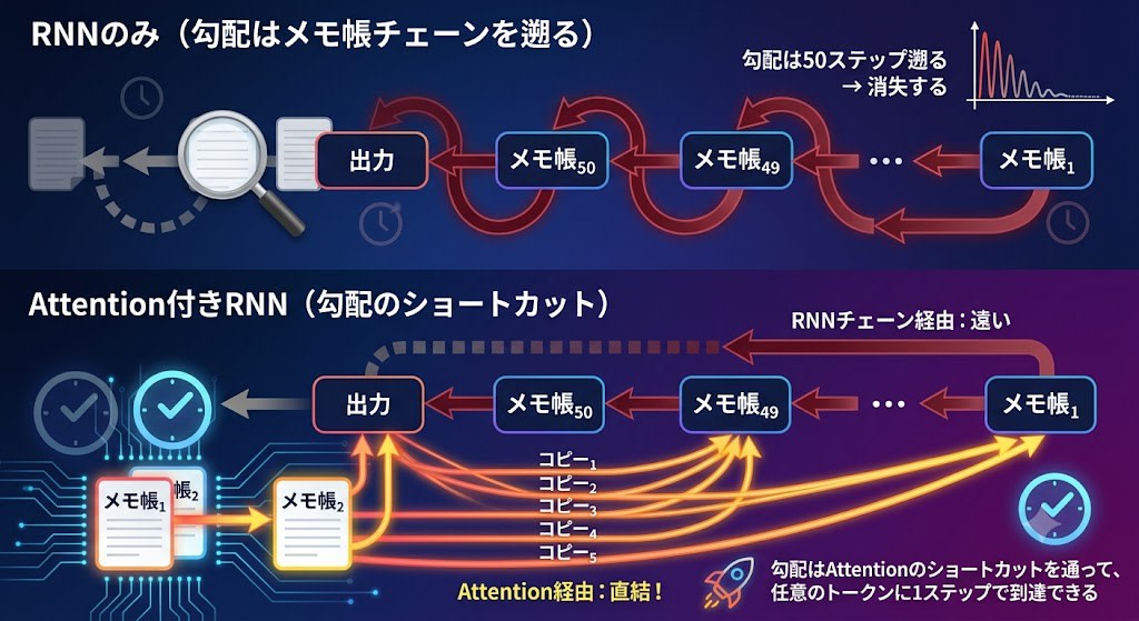
Since gradients can reach any token in one step via Attention's direct paths, there's no need to trace back through the RNN chain, and vanishing gradients are greatly mitigated.
This wasn't a grand vision. It was an engineering patch for the bug of long-sentence accuracy dropping in translation. But as a result, it solved the snapshot constraint (inability to query specific tokens) and even improved vanishing gradients.
The Patch Became an Architecture: Transformer (2017)
The question Vaswani et al. posed: "Is RNN (the sequential processing mechanism) even necessary? Can we translate with just Attention?"
Looking back at the improvements so far, even with Attention + RNN, the constraints of the RNN part remained — snapshot generation is sequential processing.
With Attention + RNN, references (re-reading) can be parallelized, but snapshot generation is still handled by the RNN. Each snapshot depends on the previous snapshot, so they can only be created in order.
Attention + RNN: references improved, but snapshot generation remains sequential

  snapshot₁ = f("The", empty)           ← calculate this first
  snapshot₂ = f("cat", snapshot₁)       ← cannot calculate until snapshot₁ is complete
  snapshot₃ = f("sat", snapshot₂)       ← cannot calculate until snapshot₂ is complete

  Each snapshot depends on the previous snapshot → chain → cannot be parallelized
Vaswani et al.'s insight was to discard this chain (the notepad chain) itself.
How to Understand Context Without RNN
In RNNs, the order of tokens was implicitly expressed through the chain of notepads. It's precisely because "The" is processed before "cat" that "cat's" notepad contains information about "The." Processing order = context order.
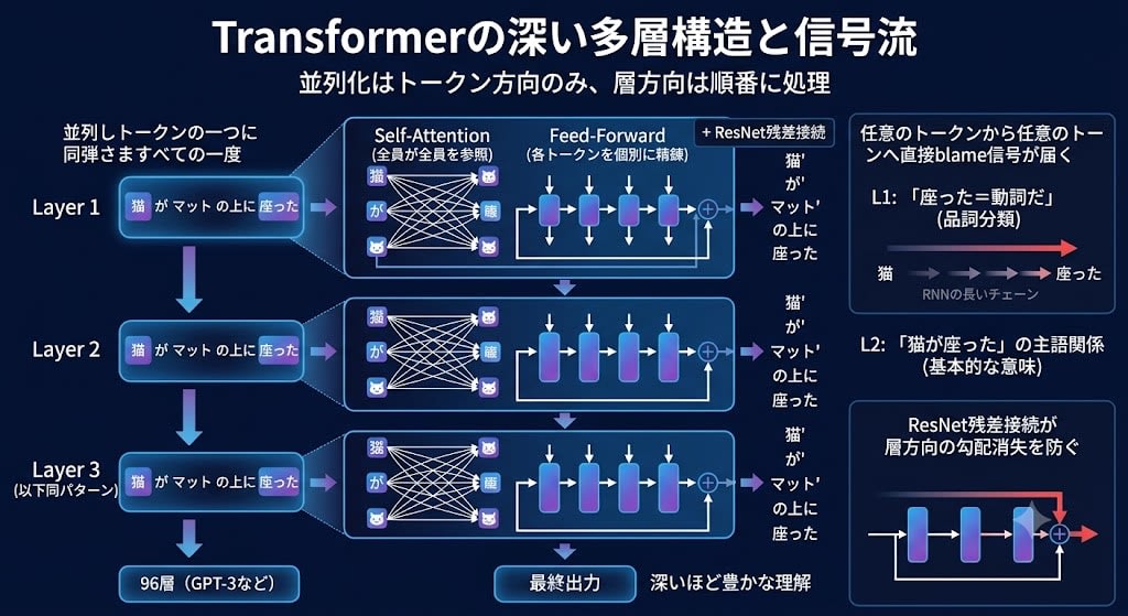
Transformer takes a completely different approach. Each token has its own position number from the start.
Since positional information is included in the data itself, order is not lost even when all tokens are processed simultaneously. And each token references all other tokens — this is the Transformer's Self-Attention.
In the earlier Attention, the mechanism was "the output RNN references snapshots of the input." In Self-Attention, input tokens reference each other. "cat" looks at "sat," and "sat" looks at "cat" — all simultaneously.
In RNNs, there was a dependency chain: "to calculate notepad₃, we need notepad₂, and notepad₂ needs notepad₁." Transformer has no such chain. Each token's Embedding doesn't depend on the processing results of other tokens — that's why they can be processed simultaneously.
Hearing "process all tokens simultaneously" might make it sound like the network became "flat." But Transformer is still a deep multi-layer structure. GPT-3 has 96 layers.
Only the token direction is parallelized. The layer direction is still processed in order.
Each layer refines representations. Layer 1 learns "sat = it's a verb," Layer 2 learns "cat is the subject of sat," and deeper layers learn complex semantic relationships. Deeper means richer understanding — the same principle as Chapter 3.
Backpropagation (blame) also flows backward through layers using the same mechanism as Chapter 3. In addition, through Self-Attention connections, blame signals can directly reach any token from any token — since there's no need to trace back through a long chain like in RNNs, vanishing gradients are greatly mitigated. And ResNet residual connections prevent vanishing gradients in the layer direction.
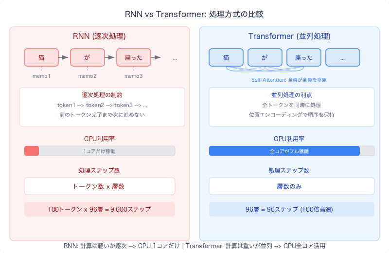
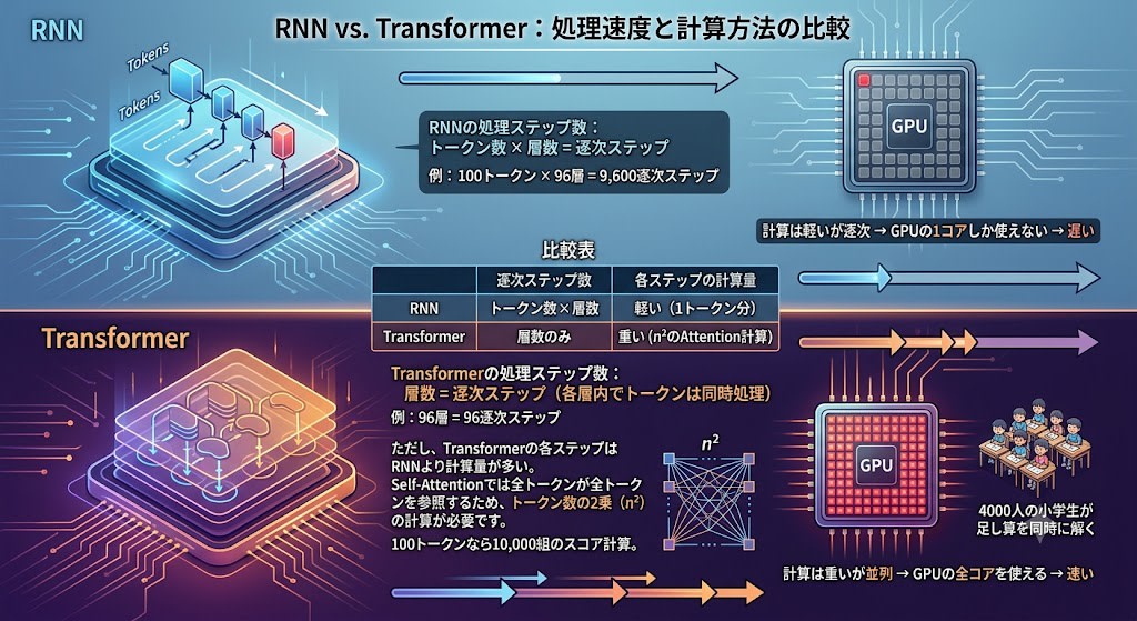
Processing Time: Why Transformer is Fast
Comparing the processing time of RNN and Transformer:
RNN's number of processing steps:
  number of tokens × number of layers = sequential steps
  example: 100 tokens × 96 layers = 9,600 sequential steps

Transformer's number of processing steps:
  number of layers = sequential steps (tokens processed simultaneously within each layer)
  example: 96 layers = 96 sequential steps
However, each step of Transformer has more computation than RNN. In Self-Attention, all tokens reference all tokens, requiring computation that is the square of the number of tokens (n²). For 100 tokens, that's 10,000 pairs of score calculations.
| Sequential steps | Computation per step | |
|---|---|---|
| RNN | tokens × layers | Light (1 token's worth) |
| Transformer | layers only | Heavy (n² Attention computation) |
The total computation can sometimes be greater for Transformer. But the heavy computation can be parallelized by GPU. This is the same structure as AlexNet in Chapter 3 — 4,000 elementary school students solving addition simultaneously. The n² score calculations are mutually independent, so they can be executed simultaneously across thousands of GPU cores.
On the other hand, the sequential steps of RNNs cannot be parallelized no matter how high-performance a GPU you have. Because you can't proceed to the next step until the previous step is complete.
As a result, Transformer solved all the problems seen in this chapter simultaneously:
| RNN | LSTM | Attention+RNN | Transformer | |
|---|---|---|---|---|
| Snapshot problem | ✗ | ✗ | ✓ (log-based) | ✓ |
| Vanishing gradient (time direction) | ✗ | ✓ (highway) | ✓ (shortcut) | ✓ (direct connection) |
| Parallel processing | ✗ | ✗ | ✗ (RNN part remains) | ✓ |
By discarding RNN and using only Attention, training became dramatically faster. Faster means being able to train larger models on more data.
An architecture aimed at improving translation speed, by enabling scale, became the foundation for all of LLMs.
Chapter 6 — Does Bigger Mean Smarter? — Scale and Emergence
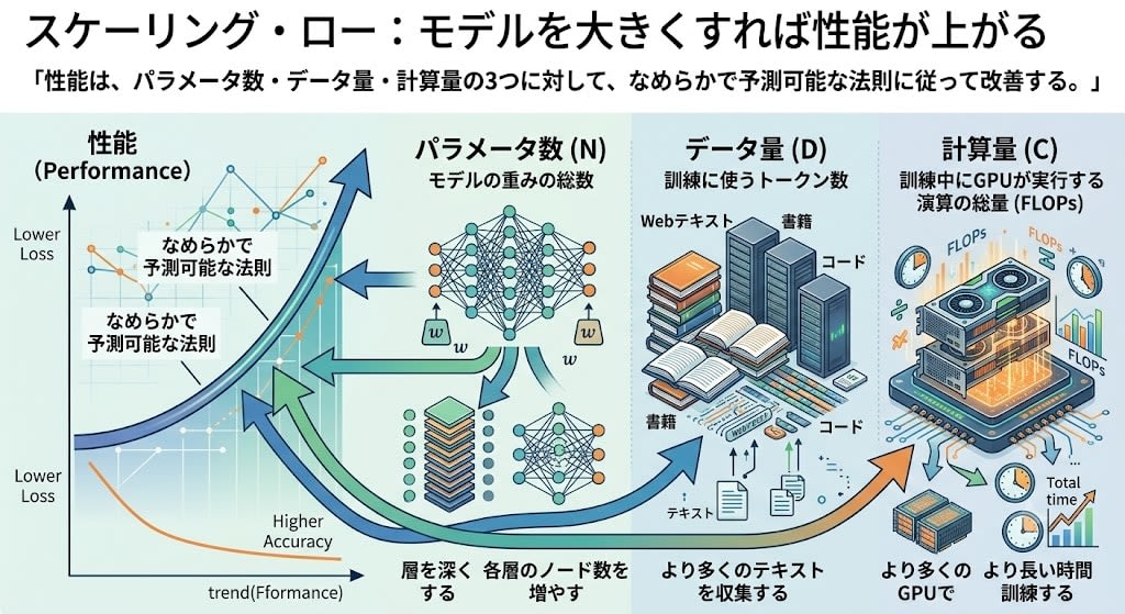
Discovery of Scaling Laws (2020)
"Increasing model size improves performance" was known as an empirical rule. Kaplan et al. at OpenAI showed this mathematically:
Performance improves according to smooth, predictable laws with respect to the three factors of parameter count, data volume, and compute.
Let's look at the three variables in detail:
| Variable | Meaning | How to increase |
|---|---|---|
| Parameter count (N) | Total number of model weights | Deepen layers, increase nodes per layer |
| Data volume (D) | Number of tokens used for training | Collect more text (web, books, code, etc.) |
| Compute (C) | Total number of operations executed by GPUs during training (FLOPs) | Train with more GPUs for longer time |
Parameter count and data volume are intuitive, but compute needs a bit of explanation.
Compute is the total number of floating-point operations (FLOPs: Floating Point Operations) executed by GPUs during training. Each time a model processes one batch, massive matrix operations run in forward propagation and backward propagation. The cumulative total of those operations is the compute.
Kaplan et al. showed the relationship between these three with an approximate formula:
That is, compute is roughly proportional to the product of parameter count and data volume. Compute is not so much an independent third variable as it is the total budget that can be invested. Once the budget is determined, it determines how large the model can be and how much data to feed it.
The way to increase compute is simple — number of GPUs × training time. Training GPT-3 consumed approximately 3.14×10²³ FLOPs. This was the result of running thousands of GPUs for weeks. In short, increasing compute means simply investing money and time.
Supplement: Chinchilla Scaling Laws (2022)
Kaplan's scaling laws suggested "when compute budget increases, more should be allocated to making the model larger." But in 2022, Hoffmann et al. at DeepMind corrected this to "more should be allocated to data volume" (Chinchilla scaling laws). The discovery was that even with the same compute budget, the optimal allocation ratio is different. What both agree on is that compute is the fundamental constrained resource.
This was a "map." It could predict in advance "if you train a model of this size with this much data, you'll get roughly this level of performance." If results are predictable, large-scale investment decisions can be made.
From Transformer to "GPT" — A Shift in Purpose
Transformer was born for translation. But GPT (Generative Pre-trained Transformer) was trying to solve a different problem from translation.
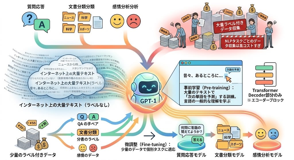
In 2018, the problem that Radford et al. at OpenAI were facing was this:
NLP has diverse tasks (question answering, document classification, sentiment analysis, etc.), but collecting large amounts of labeled data for each individual task is too costly.
There is a large amount of unlabeled text (text on the internet). Wouldn't it be good to first learn "general understanding of language" using this, and then adapt to individual tasks with a small amount of labeled data?
This is the core idea of GPT-1:
- Pre-training: Train only on "predicting the next word" using a large amount of text
- Fine-tuning: Adjust weights with a small amount of data for individual tasks
The architecture used only the Decoder part of the Transformer. The Encoder-Decoder structure for translation was unnecessary — a simple structure of "read text and predict what comes next" was sufficient.
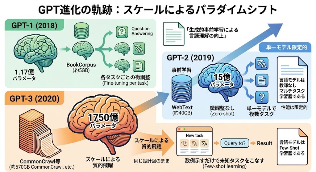
GPT-1 → GPT-2 → GPT-3: The Same Blueprint, Different Scales
This is important. GPT-1, GPT-2, and GPT-3 have nearly the same architecture. Keeping the basic design unchanged and only changing the scale to observe what happens — this is the essence of three generations.
| GPT-1 (2018) | GPT-2 (2019) | GPT-3 (2020) | |
|---|---|---|---|
| Parameter count | 117 million | 1.5 billion | 175 billion |
| Training data | BookCorpus (approx. 5GB) | WebText (approx. 40GB) | CommonCrawl etc. (approx. 570GB) |
| Core discovery | Pre-training + fine-tuning is effective | Tasks solvable without fine-tuning (Zero-shot) | Handles unknown tasks with just a few examples (Few-shot) |
| Philosophy expressed in paper title | "Improving Language Understanding by Generative Pre-Training" | "Language Models are Unsupervised Multitask Learners" | "Language Models are Few-Shot Learners" |
GPT-1 demonstrated the effectiveness of "pre-training + fine-tuning." But fine-tuning was needed for each task.
GPT-2 made the model 13 times larger and increased data. As a result, some tasks could be handled without fine-tuning (Zero-shot). As the paper title says, it was the discovery that "language models are unsupervised multitask learners." However, performance was still limited.
GPT-3 made it 117 times larger still. Architecture changes were minimal (only partial introduction of Sparse Attention). A qualitative leap occurred from scale alone, with the same blueprint.
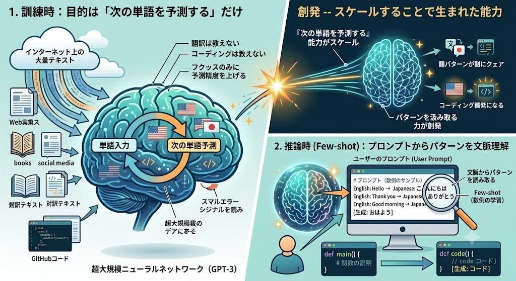
Here I'll answer a question readers might have.
"Is Few-shot part of training? Or does it happen after training?"
The answer is after training. Few-shot is a technique used at inference time (when users are using the model).
To organize GPT-3's training process:
- During training: Learn only "predict the next word" from a large amount of text collected from the internet. Translation wasn't taught, nor was coding. The only goal — improve next-word prediction accuracy
- During inference (Few-shot): Users show several sample examples in the prompt. The model reads the pattern from the context and generates continuations following the same pattern
GPT-3 was not explicitly trained in translation. However, because bilingual Japanese-English text was included in the training data, as the "next word prediction" ability scaled, the power to pick up patterns and correctly continue emerged.
Code generation is the same. Because GitHub code was included in the training data, just by showing a few examples of "function description → code," it became able to write functions it had never seen.
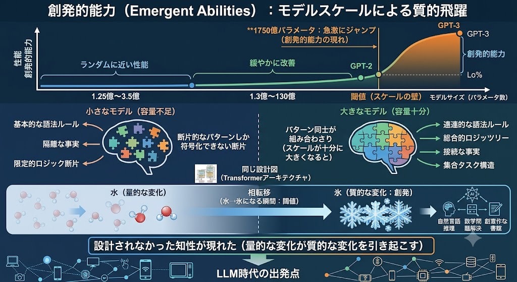
Why Did the "Big Bang" Happen with GPT-3?
Zero-shot was partially working even with GPT-2. So what changed with GPT-3?
The answer is crossing a threshold.
For many tasks, the relationship between model size and performance progressed like this:
- 125 million ~ 350 million parameters: performance close to random
- 1.3 billion ~ 13 billion parameters: gradual improvement
- 175 billion parameters: sudden jump
This is Emergent Abilities. Like a phase transition in physics (the moment water becomes ice), a quantitative change beyond a certain threshold triggers a qualitative change. GPT-2 was before that threshold, and GPT-3 was past it.
Why does a threshold exist? During training, the model encodes every pattern contained in text (grammar, logic, facts, task structure) internally in order to "predict the next word." Small models don't have enough capacity and can only learn fragments of individual patterns. But when scale becomes sufficiently large, patterns combine and abilities that weren't explicitly trained on appear on the surface — this is the nature of emergence.
GPT-3 did not design intelligence with a new architecture. As a result of scaling the same blueprint past the threshold, intelligence that wasn't designed appeared. This is the starting point of the current LLM era.
Chapter 7 — Challenges After Becoming Smart — From Fine-tuning to Alignment, and Beyond Scale
GPT-3 was remarkably versatile, but difficult to use. It would generate racist text, continue with irrelevant sentences instead of answering questions, or confidently tell lies. The ability to "predict the next word" and the ability to "give helpful answers to humans" were not the same.
The history from here is divided into three stages.
The Mechanism of Fine-tuning
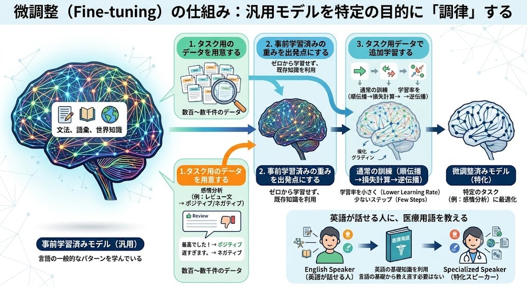
Let's look a bit more closely at fine-tuning, which appeared in GPT-1.
A pre-trained model has learned general patterns of language, but it isn't optimized for specific tasks (sentiment analysis, question answering, etc.). Fine-tuning is the process of "tuning" this general-purpose model for a specific purpose.
The mechanism is simple:
- Prepare task-specific data: For example, hundreds to thousands of pairs of "review text → positive/negative"
- Use pre-trained weights as the starting point: Rather than learning from scratch, start from weights that already understand language
- Perform additional training with task data: The same mechanism as ordinary training (forward propagation → loss calculation → backward propagation), but with a smaller learning rate and fewer steps
Why does it work with a small amount of data? Because grammar, vocabulary, and world knowledge were already acquired through pre-training. Fine-tuning is like "teaching medical terminology to someone who already speaks English" — there's no need to reteach the basics of language from scratch.
InstructGPT: "Aligning" with Human Feedback (2022)
The problem with GPT-3 was that it was "intelligent but not aligned with human intent." To solve this, OpenAI developed RLHF (Reinforcement Learning from Human Feedback), an evolution of the fine-tuning concept.
RLHF is a three-stage pipeline:
Stage 1: Supervised Fine-Tuning (SFT)
Human annotators (approximately 40 people) manually wrote around 13,000 "ideal responses" to prompts. Standard fine-tuning was applied to teach the basic behavior of "answer when asked."
Stage 2: Reward Model Training
The model generates multiple responses to the same prompt, and humans rank them by "which is better." From this ranking data, a Reward Model is trained to quantify "what constitutes a good response."
Stage 3: Optimization via Reinforcement Learning
The original model generates responses, the reward model assigns scores, and those scores are used to update the original model's weights. The model is gradually adjusted toward generating "responses humans prefer."
The results were striking. InstructGPT with 1.3 billion parameters produced responses more preferred by humans than the raw GPT-3 with 175 billion parameters. A model 130 times smaller in parameter count outperformed simply by being "aligned."
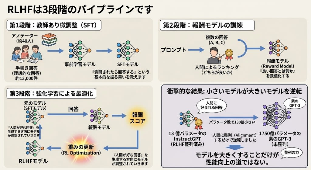
This is an important lesson: Making the model larger is not the only path to improved performance.
The Current State of Fine-Tuning: When Is It Necessary, and When Is It Not?
In the GPT-1 era, fine-tuning was required for every task. With GPT-3 enabling few-shot learning, and InstructGPT enabling zero-shot instruction-following, the role of fine-tuning has changed.
| Cases where fine-tuning is unnecessary | Cases where fine-tuning is necessary | |
|---|---|---|
| Typical examples | Email drafting, summarization, general Q&A | Medical diagnosis support, legal document review, understanding internal terminology |
| Reason | Sufficient quality with prompting a general-purpose model | Strict requirements for specialized terminology, specific formats, and compliance |
Labeled data remains important——but its purpose has changed. In the GPT-1 era, it was needed to "teach tasks," whereas today it is primarily needed to "align model behavior." The human ranking data in RLHF is a prime example.
Additionally, with the emergence of Parameter-Efficient Fine-Tuning (PEFT) methods such as LoRA (Low-Rank Adaptation) and QLoRA, it is now possible to fine-tune by adding only a small number of parameters without updating all parameters. The cost of fine-tuning has been reduced by more than 90% compared to the early 2020s.
Beyond Scale: How Are LLMs Evolving Today?
"Increase parameters, data, and compute and the model gets smarter"——the scaling laws explained GPT-3's success. However, around 2024, this strategy began hitting a wall.
Wall 1: Data Exhaustion
High-quality text data on the internet is finite. As of 2026, it is said that high-quality text written by humans has been nearly exhausted.
Wall 2: Cost Limits
Pre-training ever-larger models requires investments on the order of hundreds of millions of dollars, and diminishing returns are becoming visible.
At NeurIPS 2024, OpenAI co-founder Ilya Sutskever declared:
"Pre-training as we know it is coming to an end. The 2010s were the decade of scale. We have now returned to an era of surprise and discovery."
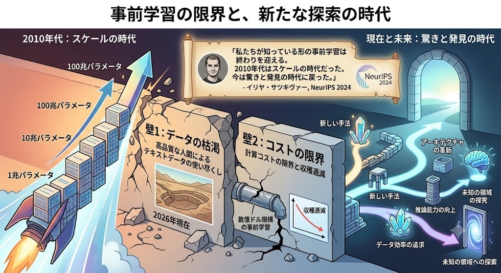
So what axes of evolution exist beyond scale? Here is an overview of the current major approaches.
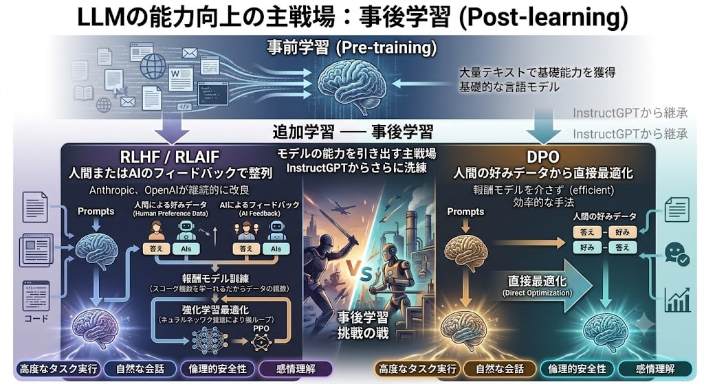
Axis 1: Deepening Post-Training
RLHF, which began with InstructGPT, has been further refined. The additional training performed after pre-training (acquiring foundational capabilities from large volumes of text)——post-training——has become the primary battleground for unlocking model capabilities.
- RLHF / RLAIF: Alignment using human or AI feedback (continuously refined by Anthropic and OpenAI)
- DPO (Direct Preference Optimization): An efficient method that optimizes directly from human preference data without going through a reward model
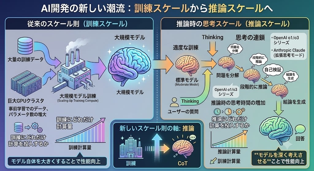
Axis 2: Test-Time Compute
Instead of scaling up training, this approach involves making the model think more at inference time.
OpenAI's o1/o3 series and Anthropic's Claude (extended thinking mode) are representative examples. The model generates a "chain of thought" before responding and reasons step by step. Rather than increasing compute at training time, performance is improved by increasing compute at inference time.
While the scaling laws governed "how much compute to invest in training," this represents a new axis of "how much compute to invest in inference."
Axis 3: Synthetic Data and Distillation
If human data is running out, have AI generate the data.
- Distillation: Training a small model (student) on responses generated by a large model (teacher). Distilled versions of DeepSeek-R1 and derived Llama models are created using this method.
- Self-Play: The model dialogues with itself, posing and solving problems to improve its own capabilities.
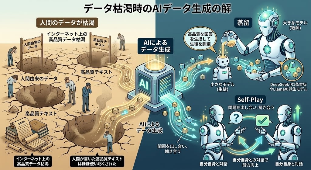
In a typical 2026 workflow, humans write 200 seed examples, a frontier model expands these to tens of thousands, quality filters are applied, and a small model is trained.
These approaches are not mutually exclusive, and current frontier models combine all three. However, the center of gravity has clearly shifted——from "bigger means smarter" to "even small models can be powerful when used wisely."
Summary: The LLM That Was Never Designed
LLMs are an accumulation of concepts developed as answers to separate problems during an era when no one was aiming to create LLMs.
Each researcher was looking only at the problem in front of them. Without a blueprint, the pieces came together over more than 80 years.
Even at this very moment, someone is stuck on an entirely different problem, and the paper they are writing to break through that wall may become a component of AI ten years from now.