I actually tried to verify satellite handover with Starlink Mini

This page has been translated by machine translation. View original
I'm Okuri, who loves whiskey, cigars, and pipes.
Through recent conversations with customers, I've started thinking that satellite links could be a viable option when high-speed communication is needed in remote locations. LEO (Low Earth Orbit) satellites like Starlink orbit at low altitudes, which means low latency and a usage experience close to terrestrial connections.
On the other hand, since LEO satellites pass overhead in just a few minutes, handovers that switch between satellites during communication are unavoidable. Research reports indicate that Starlink performs these switches every 15 seconds. I was curious about the actual impact, so I measured the connection between my Starlink Mini and an EC2 instance in the Tokyo region for one hour.
Starlink's 15-Second Cycle
The paper presented at CoNEXT 2023 above measured 4 Starlink terminals placed in the United States and Europe at high frequency, analyzing the behavior of Starlink's scheduling. The key points are as follows.
- Starlink uses a centralized control method, globally updating satellite selection, routes, and flow tables every 15 seconds
- The boundaries are aligned near the 12-second, 27-second, 42-second, and 57-second marks of each minute
From the terminal's perspective, the satellite or beam being communicated with may switch every 15 seconds. At the moment of switching, latency degradation and brief packet loss should occur, and after switching, the base latency itself should change since traffic is routed through a different satellite. Confirming these two points through actual measurement is the goal of this exercise.
Test Configuration
The configuration is as follows. A Mac measurement client is connected via wired connection to a Starlink Mini, and measurement packets are continuously sent to an EC2 instance in the Tokyo region.
[Mac (Wired LAN)]           Measurement client: irtt client / ping / starlink-grpc-tools's dish_grpc_text.py (terminal statistics)
        |
        | USB Ethernet
        v
[Starlink Mini]            192.168.100.1:9200 (gRPC)
        |
        | Satellite communication
        v
[Starlink PoP (Tokyo)]
        |
        | Internet
        v
[EC2 ap-northeast-1]       Measurement server
                           irtt server
Three types of data are measured.
| Data | Source | Granularity | What it shows |
|---|---|---|---|
| Terminal statistics (pop_ping_latency_ms / pop_ping_drop_rate) | Starlink terminal gRPC API | 1 second | Quality from antenna to PoP |
| irtt (RTT / one-way delay / loss direction) | UDP from Mac to EC2 | 100 ms | End-to-end communication status |
| ping (RTT / loss) | ICMP from Mac to EC2 | 200 ms | Verification of irtt |
The Starlink terminal exposes a gRPC API on the LAN side, and using starlink-grpc-tools allows you to extract statistics at 1-second granularity. Note, however, that this is not an officially documented API and may change with firmware updates.
irtt is a tool that sends packets at equal intervals over UDP and records one-way delay and loss direction in addition to RTT. Since behavior may differ between uplink and downlink on satellite connections, I used irtt as the primary tool rather than ping.
The key points of the configuration are as follows.
- Choosing the Tokyo region: Starlink's PoP in Japan is located in Otemachi, Tokyo. Placing EC2 in Tokyo as well minimizes the delay on the terrestrial segment, making the majority of measured values from the satellite segment.
- Connecting via wired connection: If Wi-Fi jitter is mixed in, it becomes impossible to distinguish from satellite-originated variation.
- Initiating measurements from the Starlink side: Since I have a ROAM - 100GB subscription, there is no public IP and I am behind CGNAT, making IPv4 inbound connections impossible. All measurements are initiated outbound from the Mac to EC2.
Prerequisites are as follows.
| Item | Value |
|---|---|
| Satellite antenna | Starlink Mini (mini1_pez_proto1) |
| Firmware | 2026.08.31.mr85832 |
| Installation | Outdoor location in Yokohama, Kanagawa Prefecture, clear sky, no obstructions (obstructionStats.fractionObstructed is 0, no alerts) |
| Measurement date/time | September 13, 2026, 14:45–15:47 JST (no load) |
| Measurement client | Apple M4 (macOS 26.6.2), wired connection via USB Ethernet |
| EC2 | ap-northeast-1a (apne1-az4), m8a.xlarge, Ubuntu 24.04 |
| Protocol | IPv4 |
This verification was conducted under no-load (no traffic) conditions with no data transfer. Behavior under high load with significant bandwidth consumption is out of scope.
The Starlink Mini was set up like this in practice.
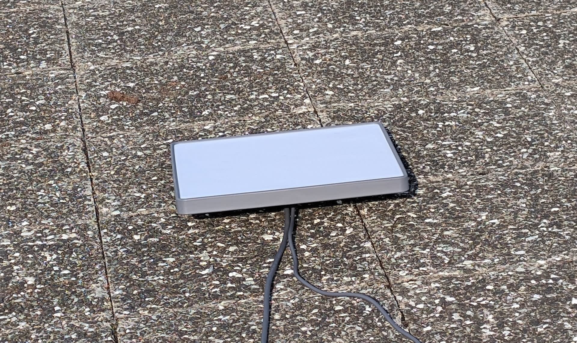
At the start of preparation, the weather looked like this (shot with a fisheye lens) — slightly cloudy — but it was mostly clear by the time measurements began.

Let's Do It
Preparing the EC2 Side
On the EC2 side, all you need to do is set up the irtt server. For the Security Group, open traffic only to the IP address confirmed via https://checkip.amazonaws.com, and only during the measurement period.
Install the necessary tools and perform time synchronization.
$ sudo apt update && sudo apt install -y irtt iperf3 chrony tmux
$ chronyc tracking
$ tmux new -d -s irtt  'irtt server -i 10ms -d 3h -l 1500'
$ tmux new -d -s iperf 'iperf3 -s'
-i 10ms is the minimum send interval permitted for clients, and -d 3h is the maximum test duration. Without changing the defaults, the server will reject long-duration, short-interval measurements, so these are relaxed.
Preparing the Mac Side
Install measurement tools via Homebrew. Since irtt doesn't appear to have a Homebrew formula, install it with go install.
$ brew install grpcurl iperf3 mtr tmux go python@3.12
$ go install github.com/heistp/irtt/cmd/irtt@latest
$ echo 'export PATH="$PATH:$HOME/go/bin:/opt/homebrew/sbin"' >> ~/.zshrc && source ~/.zshrc
Clone starlink-grpc-tools and install dependencies in a venv.
$ git clone https://github.com/sparky8512/starlink-grpc-tools.git
$ cd starlink-grpc-tools
$ python3 -m venv .venv && source .venv/bin/activate
$ pip install --upgrade -r requirements.txt
$ pip install pandas matplotlib    # For analysis
Perform time synchronization.
sudo sntp -sd time.apple.com
sntp time.apple.com
Connect the Mac to the Starlink Mini's LAN port via wired connection and verify that the gRPC API is reachable. Calling get_status with grpcurl returns the terminal's status as JSON.
$ grpcurl -plaintext -d '{"get_status":{}}' 192.168.100.1:9200 SpaceX.API.Device.Device/Handle
{
  "apiVersion": "43",
  "dishGetStatus": {
    "deviceInfo": {
      "id": "1234567890-12345678-12345678",
      "hardwareVersion": "mini1_pez_proto1",
      "softwareVersion": "2026.08.31.mr85832",
      "countryCode": "JP",
      ...
    },
    "deviceState": {
      "uptimeS": "623"
    },
    "obstructionStats": {
      "validS": 577,
      "patchesValid": 2114
    },
    "alerts": {},
    "downlinkThroughputBps": 10292.822,
    "uplinkThroughputBps": 53737.42,
    "popPingLatencyMs": 25.54012,
    "boresightElevationDeg": 81.441124,
    ...
  }
}
popPingLatencyMs is the RTT from the terminal to the PoP. It was around 25 ms under no load. The reason fractionObstructed doesn't appear in obstructionStats is that the value is 0, meaning the antenna is installed with no obstructions.
One thing I got tripped up on was Cloudflare WARP. It was installed on the client, so I disabled it along with Wi-Fi during the measurement.
Measurement Script
I prepared a script to run three measurements in parallel with tmux. Key points are as follows.
- Launch via
caffeinate -ito prevent the Mac from sleeping - macOS
pingdoesn't have Linux's-Dflag (epoch display), so use--apple-timeandTZ=UTCto add UTC timestamps to each line - Antenna statistics are appended to CSV using
dish_grpc_text.py -t 60 bulk_historyto collect only new samples every 60 seconds
run.sh
1-Minute Test Measurement
Before running for an hour, I ran it for just 1 minute to check the output.
$ ./run.sh <EC2 IPv4> 1 test
started: /path-to/measure/data/20260913T053901Z_test  (duration 1 min)
watch:   tmux ls / tail -f /path-to/measure/data/20260913T053901Z_test/irtt_v4.txt
stop:    tmux kill-server
After 1 minute, loss was zero and the median RTT was 27.49 ms. Looking at the RTT time series, there were 4 spikes, and they were neatly aligned just before 05:39:12, 05:39:27, 05:39:42, and 05:39:57. The vertical lines indicate positions where "seconds mod 15 = 12."
                         Min     Mean   Median      Max  Stddev
                         ---     ----   ------      ---  ------
                RTT  16.93ms  28.42ms  27.49ms  100.7ms  7.57ms
         send delay  22.44ms  30.88ms  30.32ms    103ms  7.42ms
      receive delay  -5.87ms  -2.46ms  -2.82ms   2.41ms  1.52ms

      IPDV (jitter)   5.71µs   5.73ms      4ms  72.44ms  7.42ms
          send IPDV   1.36µs   5.75ms   3.98ms  72.78ms  7.37ms
       receive IPDV     16ns   1.31ms    518µs    7.2ms  1.68ms

     send call time   28.3µs    113µs             340µs    31µs
        timer error    541ns    265µs            1.12ms   190µs
  server proc. time    670ns   1.15µs            8.18µs  1.04µs

                duration: 1m0s (wait 302.1ms)
   packets sent/received: 598/598 (0.00% loss)
 server packets received: 598/598 (0.00%/0.00% loss up/down)
     bytes sent/received: 102856/102856
       send/receive rate: 13.7 Kbps / 13.7 Kbps
             timer stats: 2/600 (0.33%) missed, 0.26% error
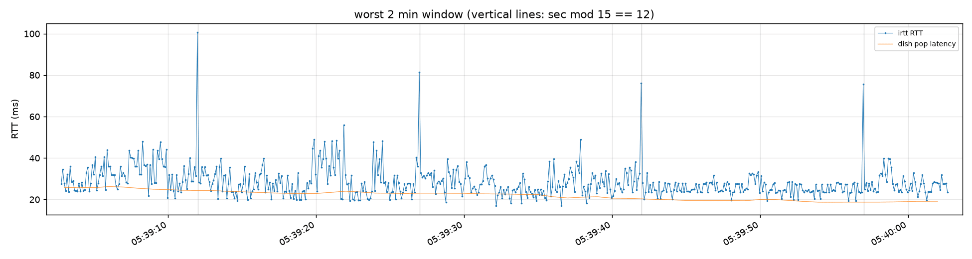
The behavior described in the paper was visible in just 1 minute. It seems worth running for a full hour.
Running for 60 Minutes
The main run is 60 minutes. It was executed during the daytime under no-load conditions.
$ ./run.sh <EC2 IPv4> 60 idle-day
started: /path-to/measure/data/20260913T054545Z_idle-day  (duration 60 min)
Then it's just a matter of waiting an hour. Since I was measuring in a spot with a clear view and no obstructions, let's enjoy some whiskey, cigars, and a pipe.
The irtt summary is as follows. Packets were sent at 100 ms intervals, with 35,957 total packets and a loss rate of 0.08%.
                          Min      Mean    Median      Max   Stddev
                          ---      ----    ------      ---   ------
                RTT   15.67ms   30.98ms   28.29ms  183.4ms   9.79ms
         send delay    9.72ms    68.5ms   76.77ms    234ms  25.61ms
      receive delay  -69.96ms  -37.52ms  -47.47ms  28.15ms   24.4ms

      IPDV (jitter)     104ns    6.51ms    4.01ms  158.9ms   8.68ms
          send IPDV     120ns    6.08ms    3.75ms  143.8ms   8.45ms
       receive IPDV      20ns    1.86ms     639µs  25.71ms   2.48ms

     send call time    13.5µs     117µs              1.2ms   26.9µs
        timer error      42ns     415µs             2.77ms    309µs
  server proc. time     300ns    1.26µs             24.6µs   1.16µs

                duration: 1h0m0s (wait 550.3ms)
   packets sent/received: 35957/35928 (0.08% loss)
 server packets received: 35934/35957 (0.06%/0.02% loss up/down)
late (out-of-order) pkts: 1 (0.00%)
     bytes sent/received: 6184604/6179616
       send/receive rate: 13.7 Kbps / 13.7 Kbps
             timer stats: 42/35999 (0.12%) missed, 0.42% error
Looking at server packets received, loss differs between uplink (antenna to EC2) at 0.06% and downlink (EC2 to antenna) at 0.02%.
Analysis
I prepared an analysis script analyze.py that cross-references the three datasets. Pass it a data directory and it generates summary.md with overall statistics, per-15-second-phase statistics, and loss run lengths formatted as Markdown tables, along with PNG graphs. The full script is long so it's on Gist.
analyze.py
$ .venv/bin/python3 analyze.py ~/measure/data/20260913T054545Z_idle-day
Here is an excerpt of the main section. It simply extracts the send timestamp and RTT from the irtt JSON, and aggregates by 15-second cycle of the send timestamp (UTC). If the behavior matches the paper's description, a peak should appear near phase 12, which is the boundary.
import json, numpy as np, pandas as pd

j = json.load(open("irtt_v4.json"))
rows = []
for rt in j["round_trips"]:
    t = rt["timestamps"]["client"]["send"]["wall"] / 1e9      # Send timestamp (UTC epoch seconds)
    rtt = rt["delay"]["rtt"] / 1e6 if "rtt" in rt.get("delay", {}) else np.nan
    rows.append({"t": t, "rtt_ms": rtt, "lost": rt["lost"] != "false"})
df = pd.DataFrame(rows)

df["phase"] = np.floor(df["t"]).astype("int64") % 15           # Seconds mod 15 = phase
print(df.groupby("phase").agg(loss_pct=("lost", lambda s: 100 * s.mean()),
                              rtt_p50=("rtt_ms", "median"),
                              rtt_p99=("rtt_ms", lambda s: s.quantile(.99))))
The terminal statistics CSV column names can be confirmed with dish_grpc_text.py -H bulk_history. Since timestamps are in UTC, converting to the same epoch seconds as irtt allows cross-referencing at second-level granularity.
Results
Overall Numbers
First, the overall statistics for the full hour.
| Measurement | Sample count | Loss rate | RTT p50 | RTT p95 | RTT p99 | RTT max |
|---|---|---|---|---|---|---|
| irtt (UDP, end-to-end) | 35,957 | 0.08% | 28.3 ms | 47.9 ms | 68.1 ms | 183.4 ms |
| ping (ICMP, end-to-end) | 17,908 | 0.10% | 25.2 ms | 43.7 ms | 58.1 ms | 145.7 ms |
| Antenna statistics (antenna to PoP, 1-second intervals) | 3,663 | 0.03% | 24.4 ms | 31.1 ms | 35.3 ms | 39.9 ms |
Looking at the median, the terminal-to-PoP segment is 24 ms and end-to-end is 25–28 ms. Since the terrestrial segment from PoP to EC2 adds only 1–4 ms, using the Tokyo region means nearly all of the measured values come from the satellite segment.
At p99, the gap between terminal statistics and end-to-end widens. This is because the antenna statistics are 1-second averages, which smooth out spikes at the 100 ms scale.
The full time series is shown below. The top panel shows RTT (blue for irtt, orange for terminal statistics), the middle panel shows loss rate, and the bottom panel shows throughput.
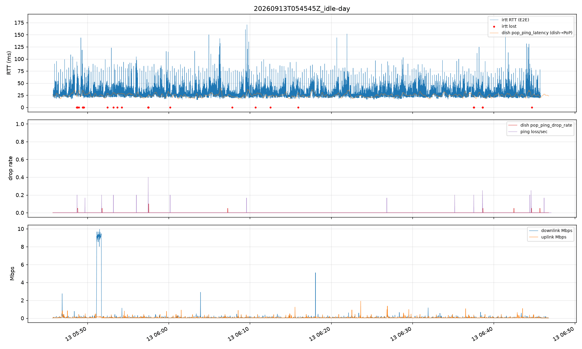
Correlation with the 15-Second Phase
The remainder when dividing the send timestamp (UTC) seconds of each sample by 15 is called the "phase," and statistics were computed per phase. If the behavior matches the paper's description, a peak should appear near phase 12, which is the boundary.
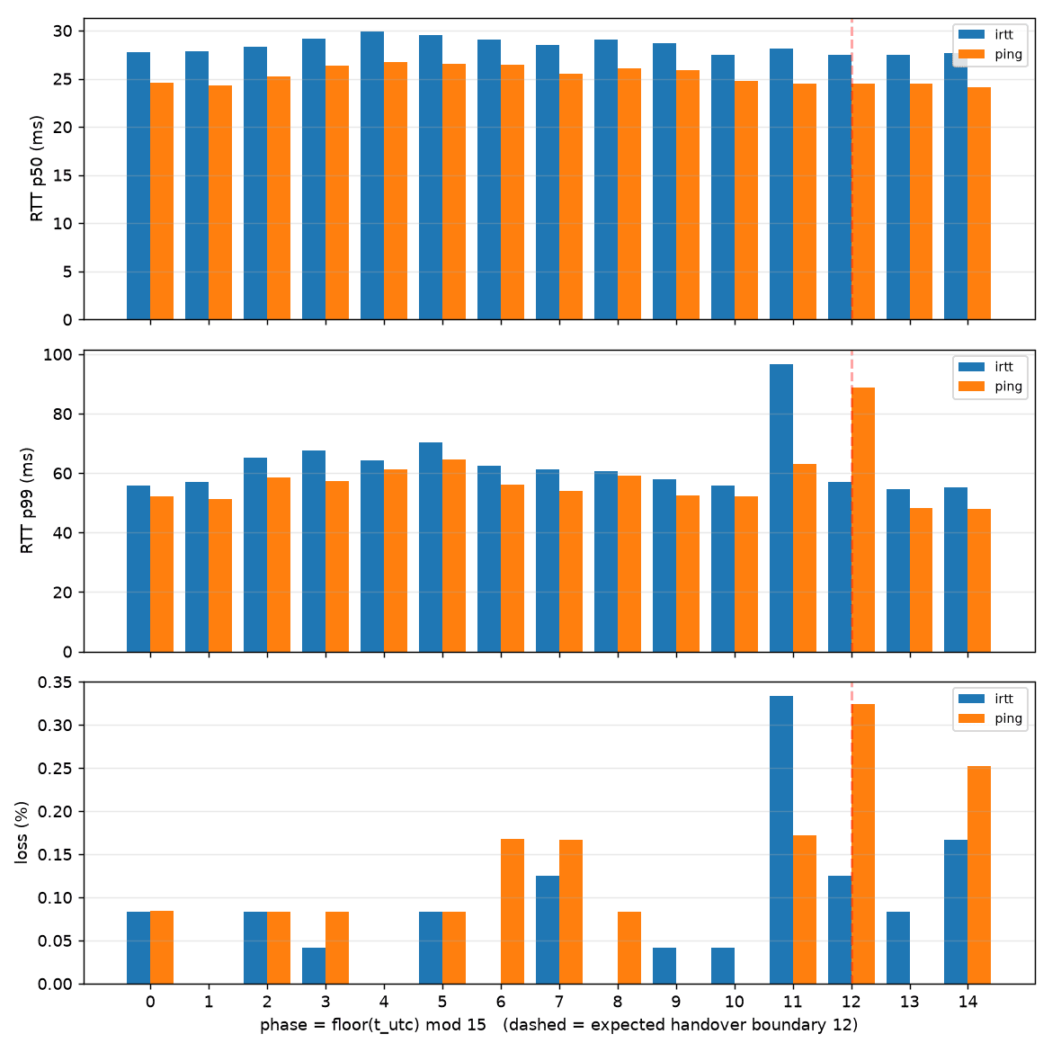
| Phase | Sample count | Loss rate | RTT p50 | RTT p99 | RTT max |
|---|---|---|---|---|---|
| 9 | 2,399 | 0.04% | 28.7 ms | 57.8 ms | 89.8 ms |
| 10 | 2,397 | 0.04% | 27.5 ms | 55.7 ms | 84.7 ms |
| 11 | 2,399 | 0.33% | 28.1 ms | 96.7 ms | 183.4 ms |
| 12 | 2,398 | 0.13% | 27.5 ms | 57.0 ms | 83.8 ms |
| 13 | 2,397 | 0.08% | 27.5 ms | 54.6 ms | 75.8 ms |
| 14 | 2,398 | 0.17% | 27.7 ms | 55.3 ms | 89.1 ms |
Only phase 11 — that is, the 1 second just before the 12-second, 27-second, 42-second, and 57-second marks — is clearly different. The RTT p99 is 96.7 ms compared to 55–70 ms for other phases, and the loss rate is 0.33% compared to 0–0.17% for other phases. The p50 is nearly constant at 27–30 ms regardless of phase, so the median doesn't change but the tail gets heavier.
The reason the peak appears 1 second before the boundary is that packets sent during phase 11 cross the boundary while traveling through the satellite and back. The same peak at phases 11 and 12 appears in ping (orange) as well, so this is not a phenomenon specific to irtt.
Zooming In for a Closer Look
The following figure zooms in on the 2-minute window with the worst loss and p99. The vertical lines indicate the 15-second boundaries (seconds mod 15 = 12).
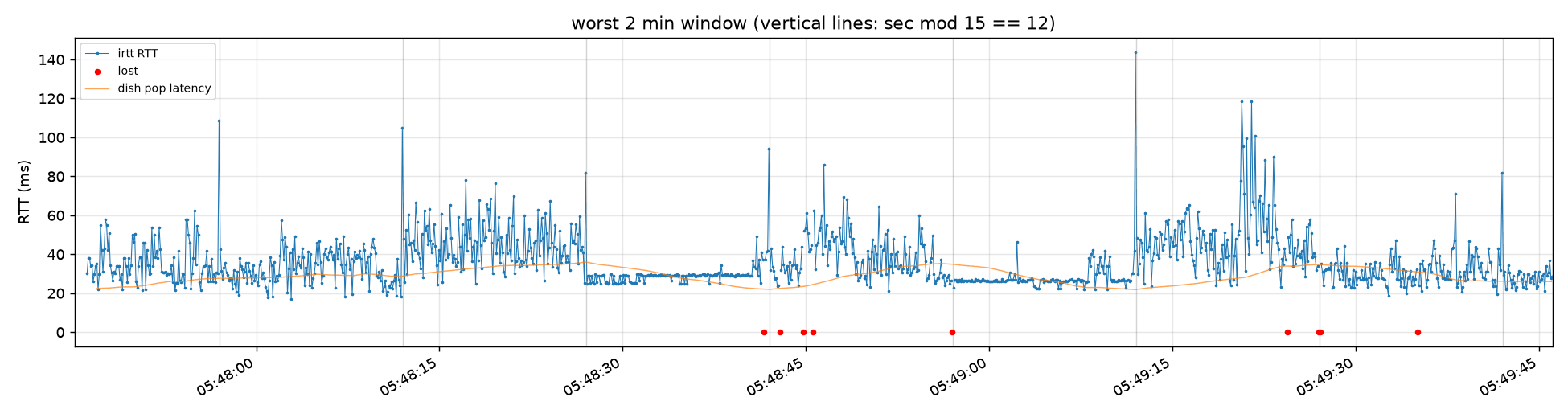
This figure reveals a characteristic pattern. Not only boundary spikes, but RTT level shifts occurring every 15 seconds are visible. At 05:48:12, it enters a noisy segment with values between 45–60 ms; at 05:48:27, it snaps cleanly to a flat segment at 27 ms; at 05:48:42, the noise returns. Every 15 seconds, the terminal is reassigned to a different satellite or beam, and the RTT level varies depending on the distance to that satellite and its congestion. The orange terminal statistics (1-second averages) gently follow the same level shifts.
How Long Does Communication Drop?
When communication is disrupted during a handover, how long does it actually last? And which direction — uplink or downlink — tends to drop? These two questions are examined using the irtt results.
First, the number of dropped packets and the number of outage events are counted separately. Since packets are sent at 100 ms intervals, grouping consecutive dropped packets into a single outage event reveals the duration of each outage.
| Item | Value |
|---|---|
| Packets sent | 35,957 |
| Dropped packets | 29 (0.08%) |
| Number of outages (consecutive losses counted as one) | 26 |
| Of which 2 consecutive packets (~200 ms) | 3 |
| 3 or more consecutive packets (300 ms or more) | 0 |
| Dropped packets falling within phases 11 and 12 | 11 (37.9%) |
The maximum outage length was 200 ms — meaning at most 2 consecutive packets dropped at 100 ms intervals — and there was not a single instance exceeding 1 second over the 60-minute period.
Looking at the phase distribution of dropped packets, phases 11 and 12 — just 2 out of 15 phases — account for 38% of all drops. Just as with the RTT spikes seen in the previous section, losses also concentrate around the handover boundaries.
Next, the direction is examined. For each packet, irtt determines: if the server didn't receive it, it's an uplink loss (Mac to EC2); if the server received it but it didn't return to the Mac, it's a downlink loss (EC2 to Mac).
| Direction | Dropped packets |
|---|---|
| Uplink (Mac to EC2) | 23 |
| Downlink (EC2 to Mac) | 6 |
Loss was skewed toward the uplink. The uplink from terminal to satellite appears to be more susceptible to switching effects. That said, the overall loss rate is 0.08%, which is at a level that should pose no problem for TCP with retransmission control.
Comparing Against International Standards
Let's compare these numbers against ITU-T Y.1541, an international standard that defines quality objectives for IP networks.
Y.1541 is a recommendation that measures IP network quality using three parameters — delay, delay variation, and loss rate — and defines upper limits that must be met per use case as "QoS classes." It serves as a common language for carriers when committing to network quality, with values defined as follows.
| Parameter | Class 0 / 1 | Class 2 / 3 | Class 4 | Class 5 |
|---|---|---|---|---|
| IPTD (IP Packet Transfer Delay) | 100 ms / 400 ms | 100 ms / 400 ms | 1 s | Not specified |
| IPDV (IP Packet Delay Variation: difference between 99.9th percentile and minimum one-way delay) | 50 ms | Not specified | Not specified | Not specified |
| IPLR (IP Packet Loss Rate) | 10⁻³ | 10⁻³ | 10⁻³ | Not specified |
| Intended use | Real-time communications sensitive to jitter such as VoIP and video conferencing | Transactions, signaling | Video streaming, bulk transfer |
Evaluation is performed per minute, and every observed minute must meet the standard. Delay variation is defined separately for uplink and downlink. Since irtt records one-way delay, uplink and downlink can be evaluated separately.
Here are the results evaluating the 60 minutes of data per minute.
| Parameter | Measured value | Verdict |
|---|---|---|
| IPTD | Average 15.5 ms (approximated as half of RTT). Even in the worst 1-minute window: 18.3 ms |
Well below Class 0's 100 ms threshold |
| IPDV (downlink) | Median 13.7 ms, maximum 50.8 ms. Exceeded 50 ms in 1 out of 60 minutes |
Almost meets Class 0/1 threshold of 50 ms |
| IPDV (uplink) | Median 64.1 ms, maximum 135 ms. Exceeded 50 ms in all 60 out of 60 minutes |
Does not meet Class 0/1 |
| IPLR | 8.1×10⁻⁴ over the full 60 minutes. On a per-minute basis, 14 out of 60 minutes exceeded 10⁻³ |
Meets Class 0–4 overall, but does not meet per-minute condition |
The absolute latency values are equivalent to Class 0. One-way delay of around 15 ms presents no significant issues compared to terrestrial fixed-line connections, and can safely be considered in a different category from geostationary satellites with one-way delays exceeding 250 ms.
On the other hand, the reason it falls short of the top Class 0/1 is delay variation, particularly uplink delay variation. Downlink variation at 14 ms stays within the Class 0 threshold, but uplink at 64 ms is 1.3 times the threshold. Combined with the earlier finding that loss was skewed toward the uplink, it seems fair to say that handover effects primarily impact the uplink direction — from the terminal toward the satellite.
Loss rate is on the borderline. The hourly average is within the threshold, but since losses concentrate around handover boundaries, one quarter of 1-minute windows exceed the threshold when evaluated per minute.
In summary, the unloaded Starlink Mini stably meets the criteria for Class 2–4 (transactions, video streaming, bulk transfer), but does not meet Class 0/1 (VoIP, video conferencing) due to uplink delay variation. This doesn't mean VoIP is unusable — rather, it means there is no guarantee of keeping variation within 50 ms at the network level as Y.1541 assumes, so the design needs to absorb it with jitter buffers on the endpoint side.
One caveat: Y.1541 requires 1,000 or more packets per minute to evaluate the 99.9th percentile, but this measurement only has approximately 600 packets at 100 ms intervals, making the per-minute loss rate evaluation particularly coarse. A re-measurement at intervals of 50 ms or less would be needed for a standards-compliant evaluation. Also, Y.1541 is fundamentally intended for evaluating carrier network quality between UNIs, so its premises differ slightly from a measurement that includes in-host processing on a Mac or EC2 as in this case.
Impact on Industrial Site Design
Applying these results to the design of connecting on-site equipment to the cloud, I think the implications are as follows. Note that the design guidelines below are estimates based on no-load measurements. Since jitter and loss rates may differ under actual workloads, load testing in a production configuration is recommended.
| Protocol / Use case | Impact of 15-second cycle | Design approach |
|---|---|---|
| General TCP (HTTPS, MQTT over TCP) | Outages of 200 ms or less are absorbed by retransmission. Throughput drops slightly due to heavier RTT | Don't set keepalive extremely short. Don't treat retransmissions of a few hundred ms as "anomalous" |
| MQTT keepalive / session | No outages exceeded 1 second, so disconnection won't occur if keepalive is set to tens of seconds | QoS 1 and persistent sessions are sufficient |
| Streaming/UDP (video, audio, some industrial protocols) | Jitter of tens to ~150 ms and losses of 100–200 ms every 15 seconds | Set jitter buffer to 200 ms or more. Use encoding and forward error correction designed to tolerate loss |
| Uplink-heavy sensor data | Loss is skewed toward the uplink | Place buffer and retransmission logic on the sending (field) side |
Caveats
- These are measurement results from using Starlink Mini at a location in Yokohama, Kanagawa Prefecture. Results may vary depending on measurement location and antenna.
- These results are from a single location, a single run, and 60 minutes of no-load measurement during the daytime. Results may vary during nighttime congestion hours or in different weather conditions.
- Measurements were taken at an installation site with no obstructions. With obstructions, obstruction-caused disconnections would mix in and become indistinguishable from handover-caused drops.
- The Starlink terminal's gRPC API is unofficial. Field names and behavior may change with firmware updates.
- Behavior when bandwidth is saturated with iperf3 is outside the scope of this measurement. I plan to cover that in a separate article.
Closing Thoughts
I've recently been interested in Amazon Leo and have been researching information about satellite communications. I had expected satellite handovers to affect communication quality, but was surprised to read in the paper that it happens as frequently as every 15 seconds. When I actually measured it, the 15-second cycle effect was clearly visible.
On the other hand, while the impact includes outages of up to 200 ms and p99 RTT of around 100 ms, a loss rate of 0.08% and average latency of around 30 ms makes this a sufficiently high-quality network connection. TCP-based protocols can be used without any special consideration, and I feel that LEO satellite communications are fully practical as a connection option for industrial sites. For UDP-based protocols sensitive to jitter and for uplink sensor data, it would be wise to design with these figures in mind.
Next, I'm thinking of writing an article summarizing the equipment needed to actually operate a Starlink Mini outdoors.