![I quickly tried making an image generation AI model [GAN]](https://devio2024-media.developers.io/image/upload/f_auto,q_auto,w_3840/v1790734566/user-gen-eyecatch/xo95hswppxjfyueh6xb4.png)
I quickly tried making an image generation AI model [GAN]

This page has been translated by machine translation. View original
Hello. My name is Kodama from the Generative AI Integration Division of the AI Business Headquarters.
I usually work as a generative AI consultant, providing proposals and support (consulting) for LLM and generative AI utilization to clients, as well as doing PM work.
In my previous job, I had experience as an ML (machine learning) engineer working on deep learning development.
While AI coding is becoming mainstream these days, in the past we used to design algorithms from scratch and do programming by hand.
Thanks to that experience, I believe I can keep up with the rapid advances in generative AI technology (mainly LLMs) at a low cost, even without following every detail.
On the flip side, for people who don't know the basics of machine learning, recent technologies must look like a complete "black box."
So, in this article, I'd like to develop an image generation AI — which likely served as a foundation for today's generative AI technologies — using the classic method called GAN, hoping to create an opportunity to understand "what generative AI actually is."
※ Please note that this adopts concepts different from the approaches that are mainstream today.
※ References are attached at the end of this article. Please refer to them as needed.
Introduction
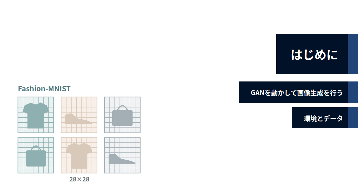
This time, to explain the mechanism of generative AI from the very basics, we will use an AI algorithm called GAN (Generative Adversarial Networks) to build a simple image generation AI.
For the AI training dataset, we will use something called Fashion-MNIST (an image dataset of fashion product photos such as T-shirts and boots).
This is an image dataset of 10 types of "fashion product" photos labeled 0 through 9, and it is often used in deep learning / machine learning research and beginner tutorials.
Using this dataset, I built a model that generates images of "non-existent clothing" using GAN.
Running GAN to Generate Images
GAN (Generative Adversarial Networks) is a method that trains two models in competition: a Generator that creates images, and a Discriminator that judges whether an image is real or fake.
For those who aren't sure what this means, there is a commonly used analogy:
A counterfeiter (generator) and a detective (discriminator) who tries to catch them both improve their skills against each other, until a counterfeit that looks just like the real thing is produced.
The mechanism will also be explained with images later, so please check it out if you want to know more.
Actually, GAN was a fairly mainstream approach in the image generation community until around 2022, when Stable Diffusion was released.
It would not be an exaggeration to say it is one of the technologies that laid the foundation for today's image generation AI.
Also, the reason I chose GAN as the subject is that its structure is simple. The Python code I implemented this time fits into about 250 lines, including the checkpoint-saving mechanism.
On the other hand, it differs from today's image generation AI in two major ways:
- Difference in generation trigger
- GAN only takes random noise as input, so you can't specify what kind of clothing will appear
- In contrast, today's image generation AI lets you specify content using text
- Difference in the approach itself
- GAN outputs an image in a single pass through the generator
- Today's image generation AI repeats the process of gradually removing noise many times
Please think of the method covered this time as appearing under the premise of "learning the basics of image generation AI."
Environment and Data
This time, we will use Fashion-MNIST as training data, Python as the programming language, and TensorFlow as the machine learning library.
Fashion-MNIST is an MIT-licensed dataset released by the research team at fashion e-commerce company Zalando.
It contains 70,000 images (60,000 for training, 10,000 for testing) of 10 types of clothing and shoes such as T-shirts, trousers, sneakers, and bags, and all images are 28×28 pixel grayscale images.
Since it is a grayscale image dataset with very few pixels and low resolution, there is no need to consider RGB and the data dimensionality is small — meaning training can be done quickly — making it perfect for tutorials.
Many of you are probably familiar with TensorFlow, but it is an open-source machine learning library developed by Google.
By using the accompanying API called Keras, it becomes easy to express complex neuron layers in code, making it possible to intuitively define neural network processing.
Here is the environment summary:
| Item | Version / Details |
|---|---|
| Language | Python 3.14 |
| Main Libraries | TensorFlow 2.21, matplotlib 3.11 (to visualize results) |
| Machine | MacBook 16GB Apple M5 (training on CPU only, no GPU) |
| Other | Claude Code |
How GAN Works
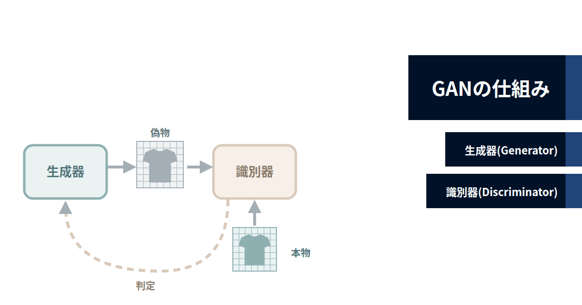
Here I'd like to explain in detail how GAN works, with images.
GAN training progresses by repeating the following 3 steps many times.
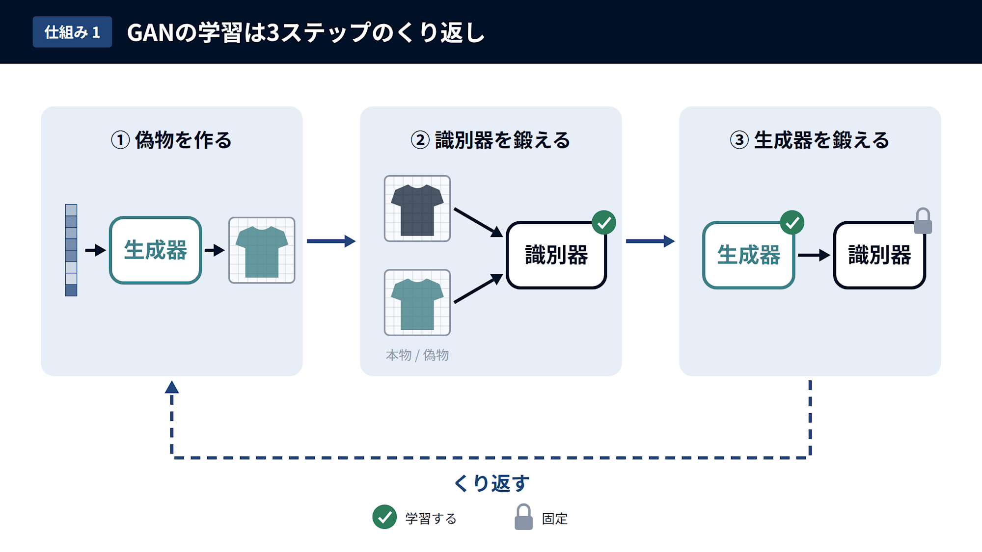
The training targets are two mechanisms: the "Generator" and the "Discriminator."
First, the process begins with a mechanism called the Generator creating a fake image from random noise. The generator before training literally produces images that look like random noise, so at this point no image with any intentional content is generated.
Next, a mechanism called the Discriminator is prepared to distinguish between real and fake images, and the noisy image from before is shown to this discriminator. (In the sense of receiving data, even if it's not literally "looking")
The discriminator is then trained to distinguish between the images it received and real images. Finally, the generator is trained to produce images that the discriminator judges as "real." Repeating this entire sequence over and over is the GAN approach.
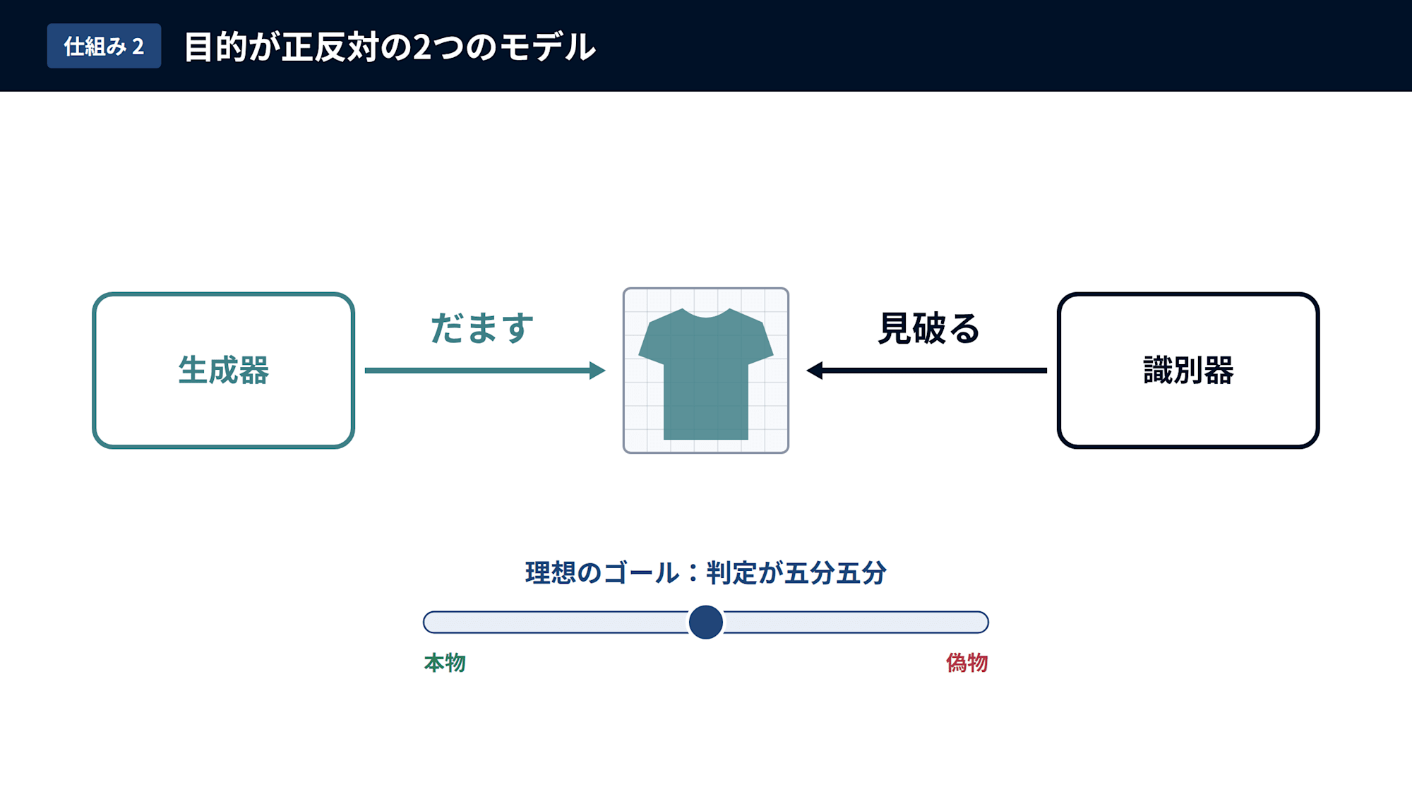
GAN is literally translated as "Generative Adversarial Network," and the reason for this comes from the fact that the roles of the generator and discriminator are complete opposites.
- Generator
- Tries to fool the discriminator
- Discriminator
- Tries to detect fakes
Since the goals of these two models are opposite, they are called "adversarial." Ideally, training settles when the generator's images become indistinguishable from real ones and the discriminator's judgment becomes a 50/50 chance.
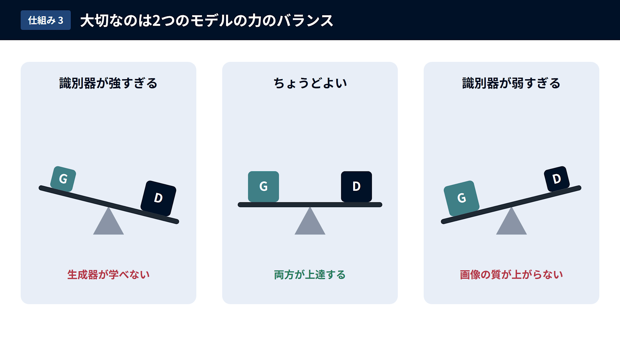
An important point when running GAN is the power balance between the two models.
For example, if the discriminator is too strong, all of the generator's images will be easily detected. Conversely, if the discriminator is too weak, even low-quality images can fool it, so the image quality won't improve.
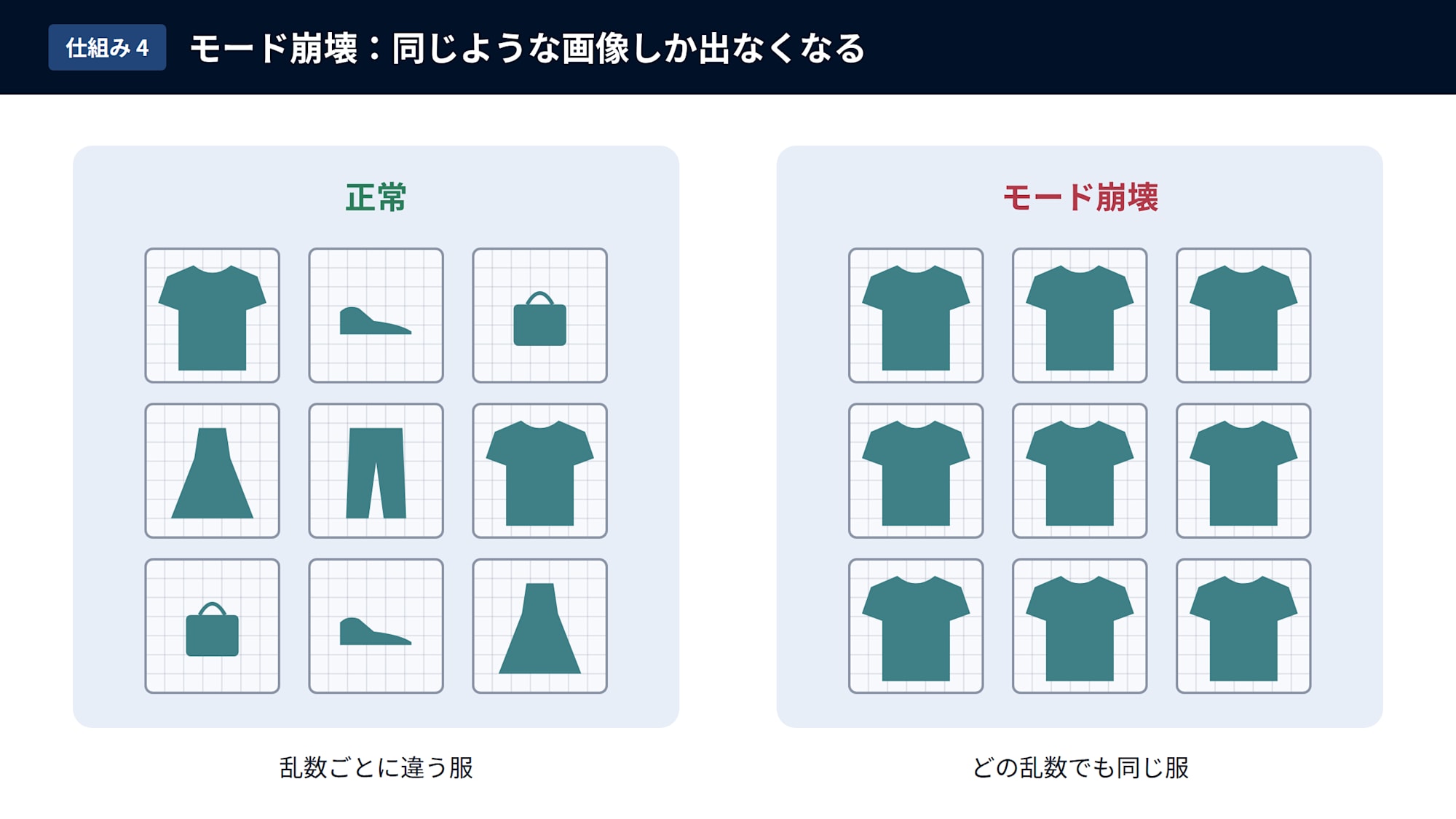
Also, the generator may start producing only images that are easy to fool the discriminator with. If things progress normally, different clothing will appear for each random input, but in this state, only similar-looking clothing will appear no matter what random input is used. This is called mode collapse.
Training generative AI models requires measures to prevent such problems.
Generator
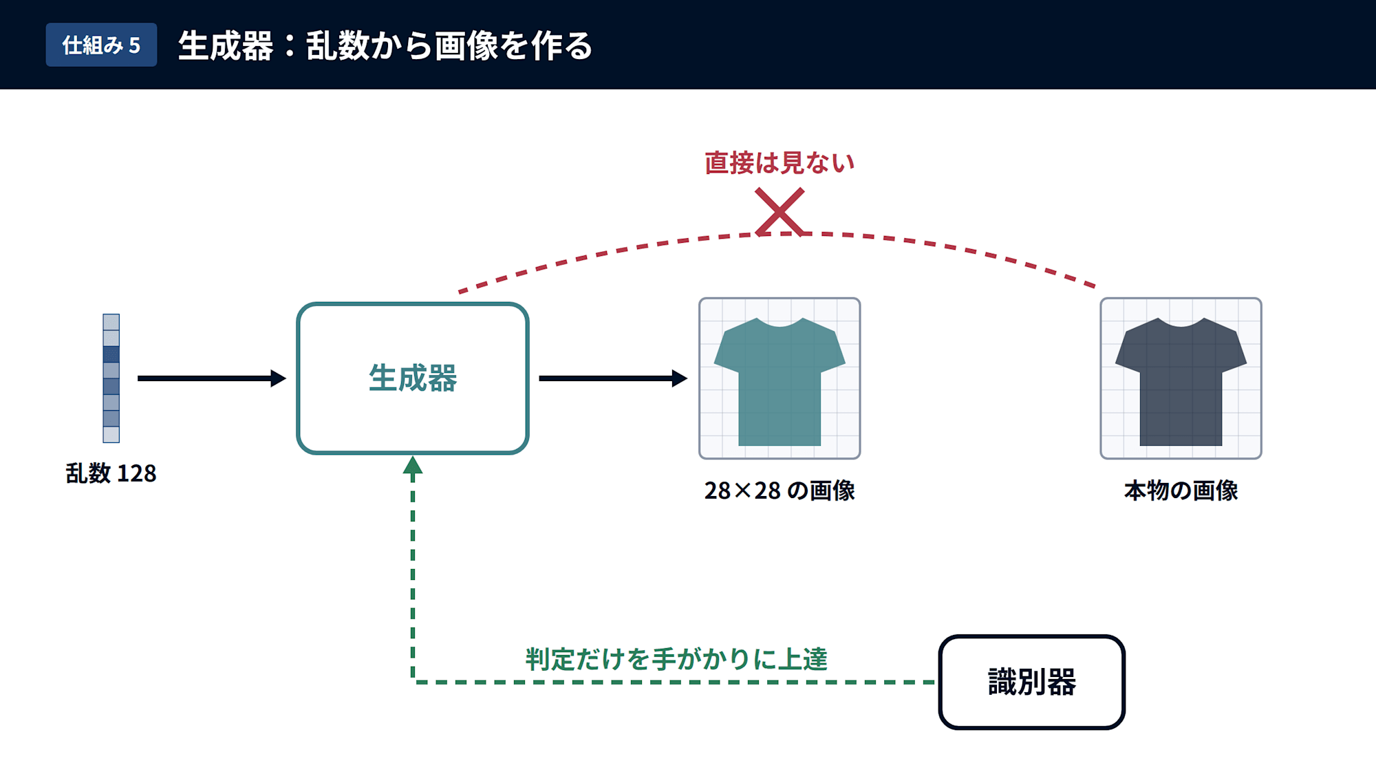
Let me explain the generator once more. In one phrase, the generator in GAN is "a model that receives random noise and outputs an image."
Before training, it can only produce noise, but as training progresses, it begins to output various clothing images depending on the random input.
This time, we create a 28×28 pixel grayscale image from a random vector of 128 numbers.
The exact number of random values doesn't matter much as long as there are enough to represent the variety of clothing in this case — results will be mostly the same whether it's slightly more or less. Anywhere from tens to hundreds should work fine, and 128 is a round number chosen from within that range.
StyleGAN, which generates high-resolution face images, often uses 512.
In any case, as shown in the figure above, the generator never directly sees real images. It improves little by little based on the discriminator's judgments.
Discriminator
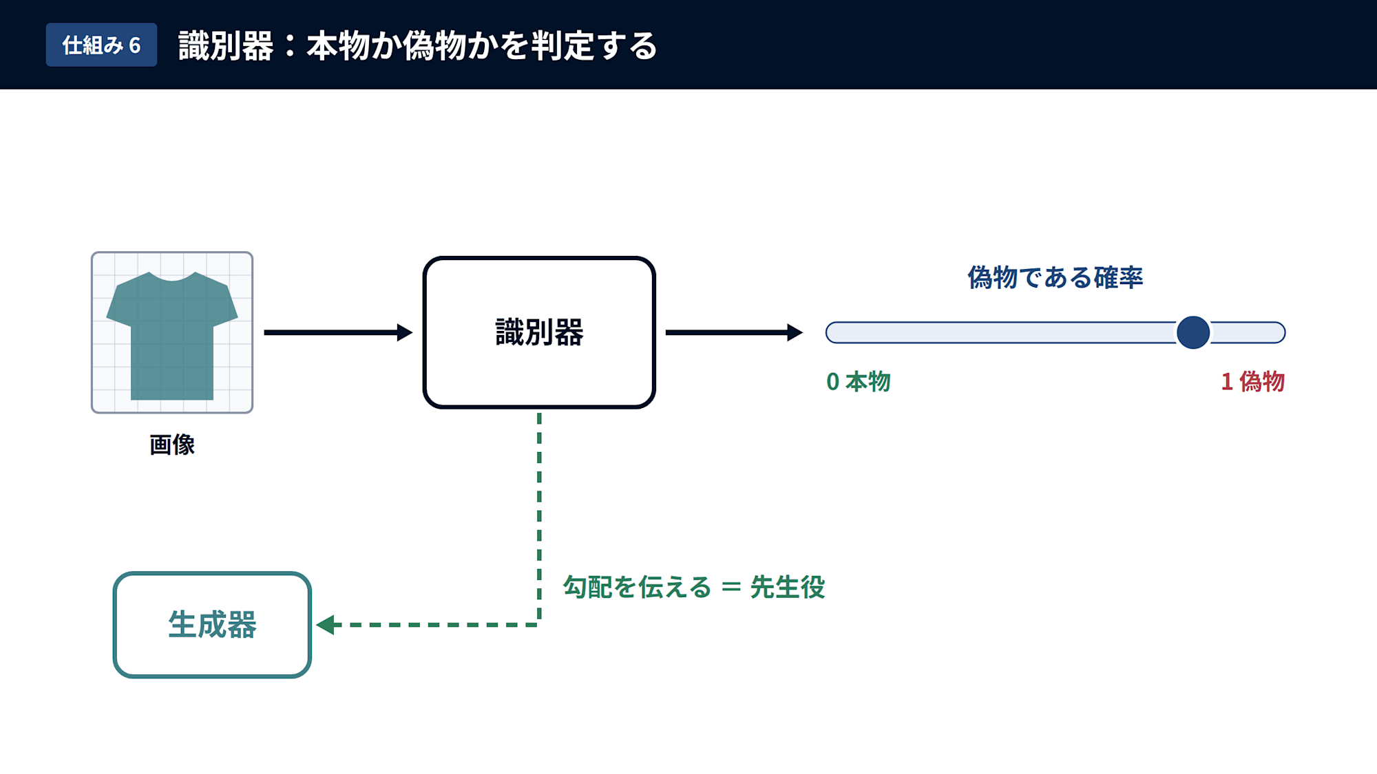
Next, I'd also like to explain the discriminator. In one phrase, it is "a model that receives an image and judges whether it is real or fake."
The discriminator outputs a number between 0 and 1 representing the probability that the image is fake. The closer to 0, the more real it judges the image; the closer to 1, the more fake.
The actual function that keeps the value in the 0–1 range is the activation function called the sigmoid function, and the reason its value represents "fakeness" is that the entire discriminator is trained with real images labeled as 0 and fake images labeled as 1.
※ Note that while many GAN explanations treat 1 as real, in this code the convention is reversed, with 0 being real.
By the way, I found a Zenn article that explains activation functions in an easy-to-understand way, so please take a look for reference.
The discriminator also plays the role of teacher for the generator.
The gradient calculated from the discriminator's judgment (a value that indicates how to adjust things to change the judgment) is passed to the generator and used for the generator's training.
In other words, if the discriminator is not a good teacher, the generator won't improve either — they are in a dependency relationship.
Let's Generate Images of Non-Existent Clothing with GAN
That's enough explanation in words — from here, let's look at the actual runnable code.
We will train a DCGAN on 60,000 training images from Fashion-MNIST, and save generated images at each epoch (one full pass through the training data, also called a generation).
The code is a single file fashion_gan.py, and you can specify the number of epochs as a command-line argument.
Training on CPU alone takes time, so even if it stops partway through, running the same command again will resume from where it left off.
※ Basically written with Claude Code, with a few manual edits.
python fashion_gan.py          # Default is 20 epochs
python fashion_gan.py 50       # Specify number of epochs
In this section, let's go through the key functions one by one.
Basic Configuration and Dataset Preparation
"""
fashion_gan.py — Generates images of "non-existent clothing" using a DCGAN trained on Fashion-MNIST.
Even if interrupted midway, running the same command again will resume from where it left off.

    python fashion_gan.py          # 20 epochs (for verification)
    python fashion_gan.py 50       # Specify number of epochs

Output (under output/):
    ckpt/            Checkpoints (latest 3 generations)
    loss.csv         Loss per epoch (epoch average, appended)
    epoch_XXXX.png   Generated image grid at the end of each epoch (always from the same random seed)
    loss.png         Loss curve
    result.png       4x4 generated image grid after training
    generator.keras / discriminator.keras

To start over, delete (or rename) the output/ folder before running.
"""

import csv
import os
import signal
import sys

import tensorflow as tf
from matplotlib import pyplot as plt
from tensorflow.keras import Model, Sequential, callbacks, layers, losses, metrics, optimizers

# ---------------------------------------------------------------- Settings
NOISE_DIM = 128          # Number of random values fed into the generator
BATCH_SIZE = 128         # Number of images trained at once
EPOCHS = int(sys.argv[1]) if len(sys.argv) > 1 else 20
OUT = "output"           # For Colab, use a path on Google Drive (e.g. /content/drive/MyDrive/fashion_gan/output)
SAVE_EVERY_STEPS = 50    # How many steps between checkpoints
os.makedirs(OUT, exist_ok=True)

for gpu in tf.config.list_physical_devices("GPU"):
    tf.config.experimental.set_memory_growth(gpu, True)

# ---------------------------------------------------------------- Data
def load_dataset() -> tf.data.Dataset:
    """Load Fashion-MNIST, normalize to -1~1, and return as a training pipeline."""
    (x, _), _ = tf.keras.datasets.fashion_mnist.load_data()
    x = (x[..., None].astype("float32") - 127.5) / 127.5  # (60000, 28, 28, 1), values are -1~1
    return (
        tf.data.Dataset.from_tensor_slices(x)
        .shuffle(len(x))
        .batch(BATCH_SIZE, drop_remainder=True)
        .prefetch(tf.data.AUTOTUNE)
    )
First, we import the necessary classes and functions from the tensorflow package.
In the settings section, we determine things like the number of random values fed into the generator (NOISE_DIM), the number of images trained at once (BATCH_SIZE), and the number of epochs (EPOCHS).
SAVE_EVERY_STEPS is the checkpoint interval — the model is saved every 50 steps (equivalent to 6,400 images).
The load_dataset function loads the training images from Fashion-MNIST.
The content of tf.keras.datasets.fashion_mnist.load_data() can be rephrased as follows:
((training images, training labels), (test images, test labels))
Each part looks like this:
| Content | Shape |
|---|---|
| Training images | (60000, 28, 28) |
| Training labels (numbers 0–9 representing clothing type) | (60000,) |
| Test images and test labels | (10000, 28, 28) and (10000,) |
In other words, 60,000 28×28 pixel images and their corresponding labels are divided into "training" and "test" sets.
Since we only use the training images, we receive them in x, and discard the unused labels and test data with _.
For a good explanation of why training and test data are separated, I found another helpful Zenn article, so please take a look.
The x[..., None] part adds a channel dimension so that it can be accepted by convolutional layers, changing the image shape to (60000, 28, 28, 1).
The subsequent (x - 127.5) / 127.5 is a normalization step that maps pixel values from 0–255 to the range -1–1.
(0 becomes -1, 127.5 becomes 0, 255 becomes 1)
The reason for using -1–1 instead of 0–1 is that the generator's output, which appears later, is in the range of -1–1.
Preparing the Generator
# ---------------------------------------------------------------- Models
def build_generator() -> Sequential:
    """Random vector → 28x28x1 image (-1~1). Upsample twice from 7x7 to reach 28x28."""
    return Sequential(
        [
            layers.Input((NOISE_DIM,)),
            # 128 → 7x7x128 (no bias needed directly before BatchNormalization)
            layers.Dense(7 * 7 * 128, use_bias=False),
            layers.BatchNormalization(),
            layers.LeakyReLU(0.2),
            layers.Reshape((7, 7, 128)),
            # 7x7x128 → 14x14x128
            layers.UpSampling2D(),
            layers.Conv2D(128, 5, padding="same", use_bias=False),
            layers.BatchNormalization(),
            layers.LeakyReLU(0.2),
            # 14x14x128 → 28x28x64
            layers.UpSampling2D(),
            layers.Conv2D(64, 5, padding="same", use_bias=False),
            layers.BatchNormalization(),
            layers.LeakyReLU(0.2),
            # 28x28x64 → 28x28x1 (tanh constrains pixel values to -1~1)
            layers.Conv2D(1, 5, padding="same", activation="tanh"),
        ],
        name="generator",
    )
The generator in this case is a model that creates a 28×28 grayscale image from 128 random values. The overall flow is as shown in the figure below, where a small feature map is enlarged twice to reach the image size.
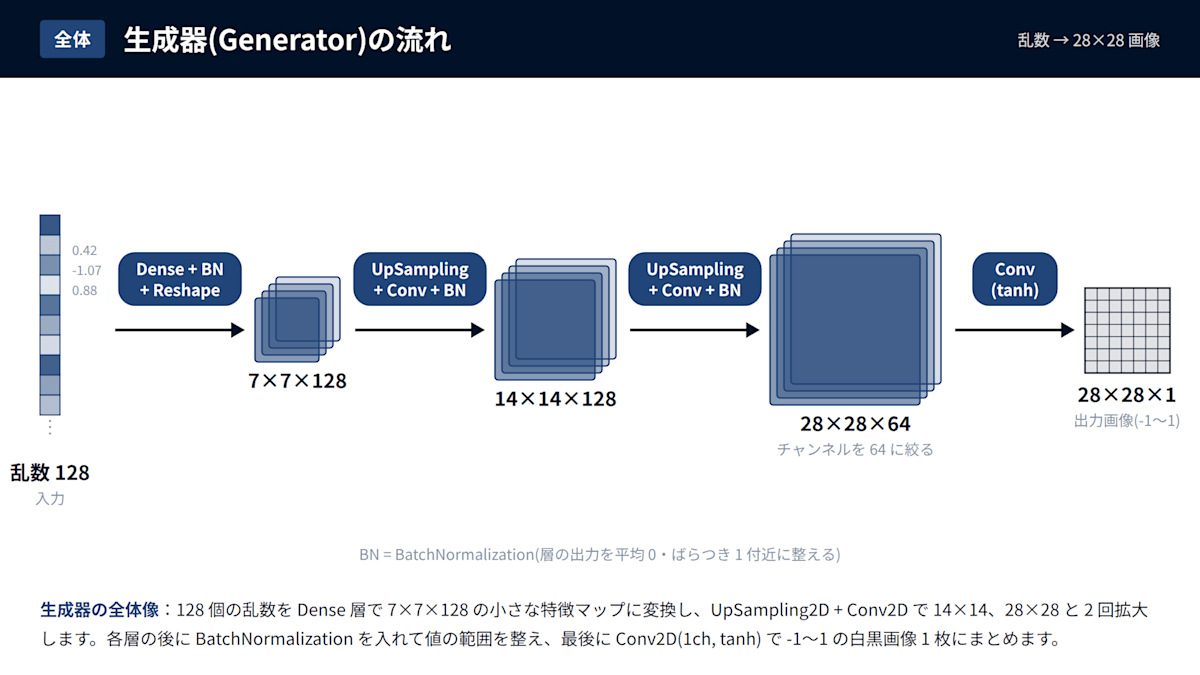
What this upsampling (UpSampling) is doing is enlarging the vertical and horizontal size of the image (feature map).
This will be explained in Step 2 later, so please refer to it then.
Another element, BatchNormalization, which appears after each layer, is a process that normalizes the values coming out of a layer so that, for each batch (128 images), the mean is around 0 and the variance is around 1.
GAN training tends to collapse if values become extremely large or if everything sticks to the same value during training, so keeping the value range organized at each layer stabilizes training.
For this reason, it is important to insert batch normalization throughout.
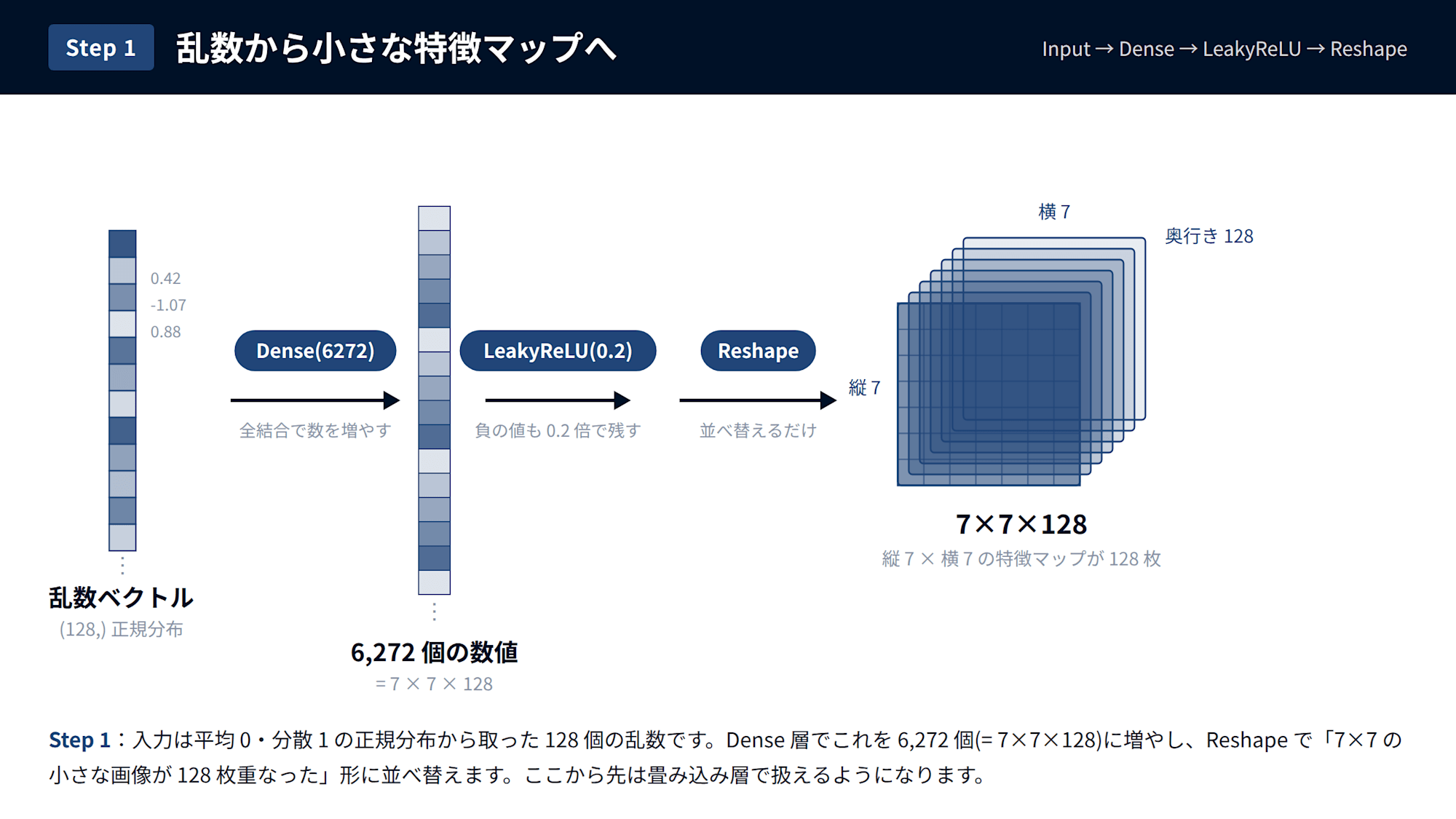
First, the 128 random values are expanded by Dense to 6,272 values (= 7×7×128), the value range is normalized by BatchNormalization, and then Reshape rearranges them into the shape of "128 small 7×7 images stacked on top of each other."
At this point it still can't be called an image, but since it's now in a 3D shape of height × width × channels (number of stacked feature maps), it can be handled by convolutional layers from here on.
The use_bias=False on Dense and Conv2D is a setting that disables the "bias" — a uniform value added to the output.
Since the immediately following BatchNormalization resets the mean to 0, any added value would be cancelled out, making it meaningless to have a bias.
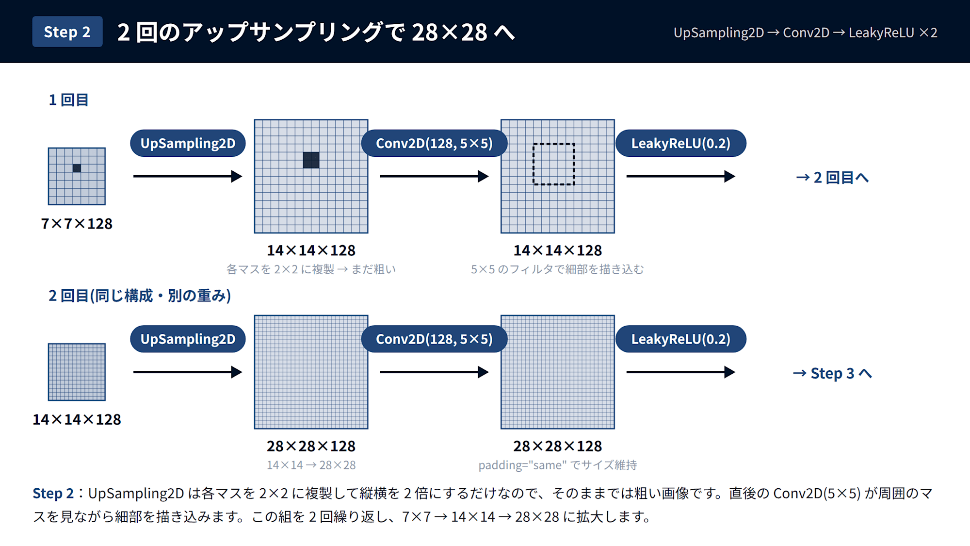
Next, the UpSampling2D layer duplicates each cell into a 2×2 block, doubling the height and width.
Upsampling is the process of increasing the vertical and horizontal size of an image like this.
However, since simply duplicating cells results in a rough image, the subsequent Conv2D fills in the details by looking at surrounding cells, as shown by the dotted outline in the figure.
By repeating this process twice, the image is enlarged from 7×7 → 14×14 → 28×28, increasing the resolution of the image.
The number of channels decreases from 128 on the first pass to 64 on the second, as resolution increases. Since the computation increases as the size grows, the number of channels is reduced accordingly to maintain balance.
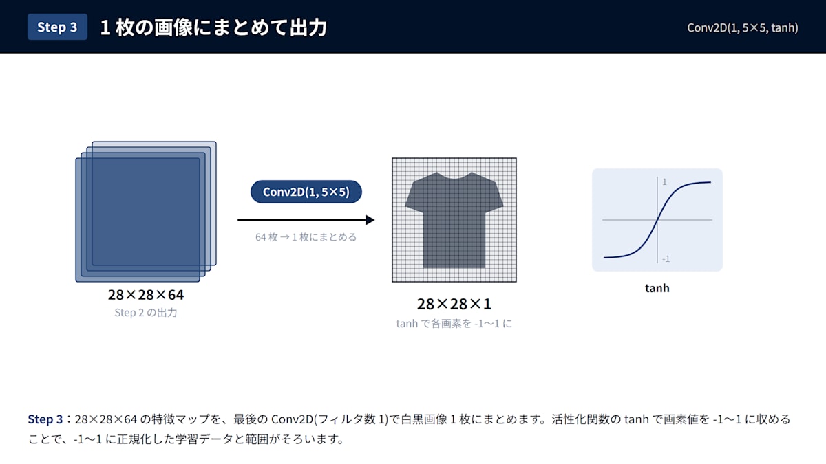
Finally, the 28×28×64 feature map is combined into a single grayscale image with a filter count of 1 using the final Conv2D.
The activation function tanh is used to keep pixel values in the range of -1–1. This aligns the range with the training data that was normalized to -1–1.
The activation function LeakyReLU used at each step retains a slope of 0.2 for negative values to prevent gradients from dying out, and is commonly used in GANs.
Preparing the Discriminator
def build_discriminator() -> Sequential:
    """28x28x1 image → probability of being fake (0=real, 1=fake)."""
    return Sequential(
        [
            layers.Input((28, 28, 1)),
            # 28x28x1 → 14x14x64 (stride 2 halves height and width)
            layers.Conv2D(64, 5, strides=2, padding="same"),
            layers.LeakyReLU(0.2),
            layers.Dropout(0.3),
            # 14x14x64 → 7x7x128
            layers.Conv2D(128, 5, strides=2, padding="same"),
            layers.LeakyReLU(0.2),
            layers.Dropout(0.3),
            # 7x7x128 → 6,272 → 1
            layers.Flatten(),
            layers.Dense(1, activation="sigmoid"),
        ],
        name="discriminator",
    )
The discriminator in this case is a model that receives a 28×28 image and outputs a single value representing the "probability that it is fake."
The overall flow is as shown in the figure below, and it works in exactly the opposite direction to the generator — shrinking the image while increasing the features.
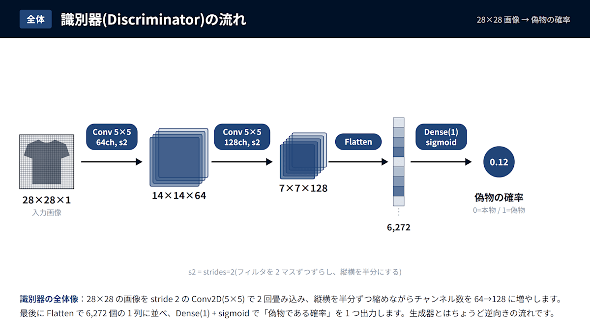
What the central convolution (Conv2D) is doing is sliding a small window (filter) across the image step by step, picking out features such as lines and edges.
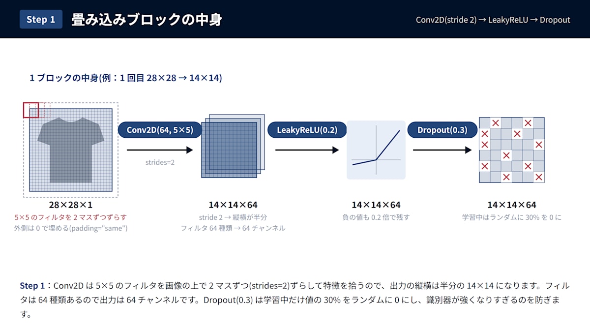
First, let's look at one block consisting of Conv2D, LeakyReLU, and Dropout, and what happens inside it.
Conv2D slides a 5×5 filter across the image to pick up features.
In the code, strides are set to 2, meaning the filter moves 2 cells at a time instead of 1, so the output dimensions shrink from 28×28 to 14×14.
Dropout is a mechanism that randomly sets x% of the values output by the layer to 0 (drops them out).
As mentioned earlier, "the most important thing when running GAN is the power balance between the two models" — if the discriminator becomes too strong by memorizing the training data, the generator can no longer learn, so this kind of mechanism is necessary.
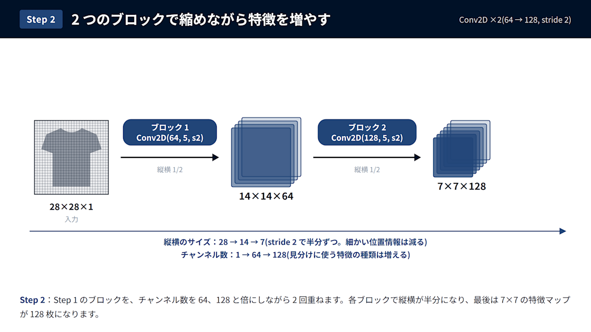
Next, the block constructed above is stacked twice, with the number of channels doubling to 64 and then 128.
While the spatial dimensions shrink from 28→14→7 by halving each time, the number of channels increases from 1→64→128.
Since halving the height and width reduces the number of cells to one-quarter, the number of channels is increased proportionally to expand the variety of features used for discrimination.
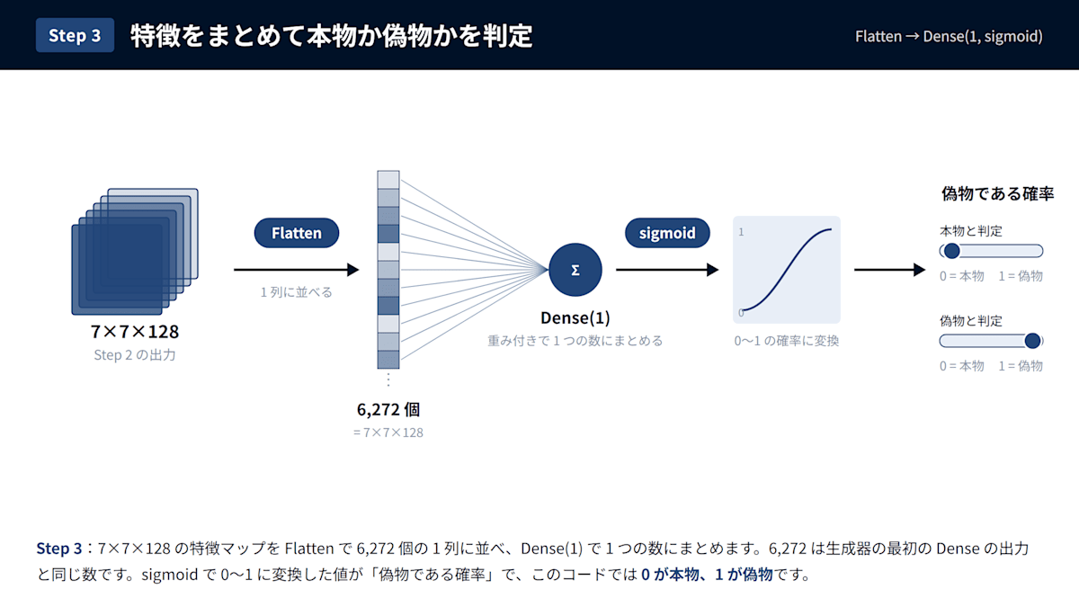
Finally, the features collected so far are gathered together to produce the final judgment.
Flatten is a layer that rearranges the 7×7×128 feature map into a flat list of 6,272 values.
The next Dense layer multiplies each of the values in the flat list by a weight and sums them, so it requires vector-form input (it cannot accept the 3D shape of height × width × channels).
That's why Flatten is used — it changes only the arrangement without performing any computation, putting the data into a form that can be passed to Dense. It is the inverse of Reshape in the generator, and the number 6,272 happens to match the initial 6,272 values in the generator.
After that, Dense multiplies the 6,272 values by weights, sums them up, and consolidates them into a single value.
The value produced by the final sigmoid, constrained to the range 0–1, represents the probability that the image is fake.
The sigmoid function, unlike a hard 0 or 1 choice, can output intermediate values like 0.12 or 0.87 as a non-linear layer, allowing it to express "how fake-like" an image is in a gradated manner.
Preparing the Training Step
# ---------------------------------------------------------------- GAN
class GAN(Model):
    """Trains the generator and discriminator alternately. Labels are 0=real, 1=fake."""

    def __init__(self, generator, discriminator):
        super().__init__()
        self.g, self.d = generator, discriminator
        self.g_opt = optimizers.Adam(2e-4, beta_1=0.5)
        self.d_opt = optimizers.Adam(2e-4, beta_1=0.5)
        self.bce = losses.BinaryCrossentropy()
        # Containers for averaging loss within an epoch (auto-reset at the start of each epoch)
        self.d_loss_tracker = metrics.Mean(name="d_loss")
        self.g_loss_tracker = metrics.Mean(name="g_loss")
        self.compile()

        # Checkpoint targets: weights, Adam internal state, number of completed epochs
        self.epoch = tf.Variable(0, dtype=tf.int64)
        self.ckpt = tf.train.Checkpoint(
            g=self.g, d=self.d, g_opt=self.g_opt, d_opt=self.d_opt, epoch=self.epoch
        )
        self.ckpt_manager = tf.train.CheckpointManager(self.ckpt, f"{OUT}/ckpt", max_to_keep=3)

    @property
    def metrics(self):
        return [self.d_loss_tracker, self.g_loss_tracker]

    def save_ckpt(self):
        self.ckpt_manager.save()

    def restore(self) -> int:
        """Try loading from the newest checkpoint, and return the number of completed epochs. Returns 0 if no checkpoint exists."""
        for path in reversed(self.ckpt_manager.checkpoints):
            try:
                self.ckpt.restore(path).expect_partial()
                print(f"resumed from {path} (epoch {int(self.epoch)} done)")
                return int(self.epoch)
            except Exception as e:  # Skip checkpoints that were corrupted by mid-write interruption
                print(f"skip broken checkpoint {path}: {e}")
        self.epoch.assign(0)
        return 0

    def train_step(self, real):
        n = tf.shape(real)[0]
        noise = lambda: tf.random.normal((n, NOISE_DIM))

        # Discriminator: train to judge real→0, fake→1
        # Only the real labels are shifted to 0~0.1 to suppress overconfidence in the discriminator (one-sided label smoothing)
        # The generator is called with training=True to keep BatchNormalization in training mode (weights are not updated)
        fake = self.g(noise(), training=True)
        with tf.GradientTape() as tape:
            pred = tf.concat([self.d(real, training=True), self.d(fake, training=True)], 0)
            label = tf.concat([0.1 * tf.random.uniform((n, 1)), tf.ones((n, 1))], 0)
            d_loss = self.bce(label, pred)
        self.d_opt.apply_gradients(zip(tape.gradient(d_loss, self.d.trainable_variables), self.d.trainable_variables))

        # Generator: train to make the discriminator misclassify its images as "real (0)"
        with tf.GradientTape() as tape:
            pred = self.d(self.g(noise(), training=True), training=False)
            g_loss = self.bce(tf.zeros_like(pred), pred)
        self.g_opt.apply_gradients(zip(tape.gradient(g_loss, self.g.trainable_variables), self.g.trainable_variables))

        self.d_loss_tracker.update_state(d_loss)
        self.g_loss_tracker.update_state(g_loss)
        return {"d_loss": self.d_loss_tracker.result(), "g_loss": self.g_loss_tracker.result()}
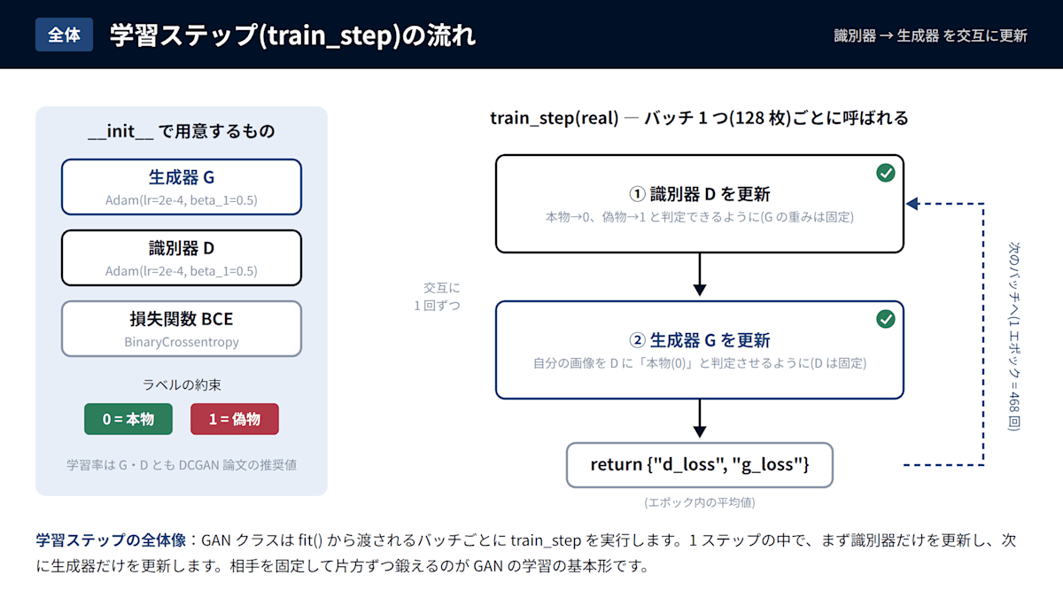
The GAN class was created to bundle the generator and discriminator together and allow training via Keras's fit function.
It inherits from Keras's Model class and overrides train_step, so calling fit() automatically executes GAN-specific training for each batch. The overall flow is as shown in the figure below.
What the loss here is doing is expressing "how far the model's answer is from the correct answer" as a single number.
Training an AI model means, in short, gradually moving the weights in the direction that reduces this loss.
First, in __init__ on the left of the figure, the tools for training are prepared.
Separate optimizers (Adam) are prepared for the generator and discriminator respectively, with a learning rate of 2e-4 (0.0002) for both.
beta_1=0.5 is the value that controls "how much Adam carries forward the direction of past gradients," and it is set lower than the standard 0.9. In GAN, because the opposing model changes slightly with every step, this is set lower so that the current model isn't pulled too strongly by past directions and can adapt quickly to the current situation.
The loss function is binary cross-entropy (BCE), commonly used for binary classification problems. The convention here is that 0 is real and 1 is fake.
d_loss_tracker and g_loss_tracker are containers for averaging the loss within an epoch. Since the per-batch loss tends to fluctuate, this allows us to observe the trend over the entire epoch average.
The right side of the figure shows the inside of train_step, where one "discriminator update" and one "generator update" are performed in this order for each batch (128 images).
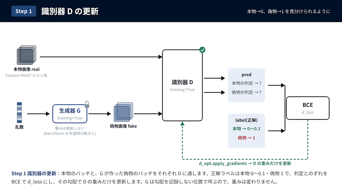
At the beginning of the training step, the discriminator is updated.
The upper part of the figure is the flow for real images, and the lower part is for fake images — both are passed through the discriminator to produce predictions (pred).
The generator that creates fake images is called outside the tape that records gradients, so the generator's weights are not changed at all at this stage.
The reason for calling it with training=True is to keep the BatchNormalization inside the generator behaving as it does during training (normalizing values using the mean and variance of the current batch).
The ground-truth labels are 0 for real and 1 for fake.
On top of that, only the real labels are randomly shifted to the range 0–0.1. This is to prevent the discriminator from being too confident about "definitely real," and is a technique known as Label Smoothing.
The value obtained by computing the discrepancy between the predictions and the correct labels using BCE is d_loss.
tape.gradient computes "which weights should move in which direction to reduce d_loss," and only the discriminator's weights are updated, as shown by the green dashed line in the figure.
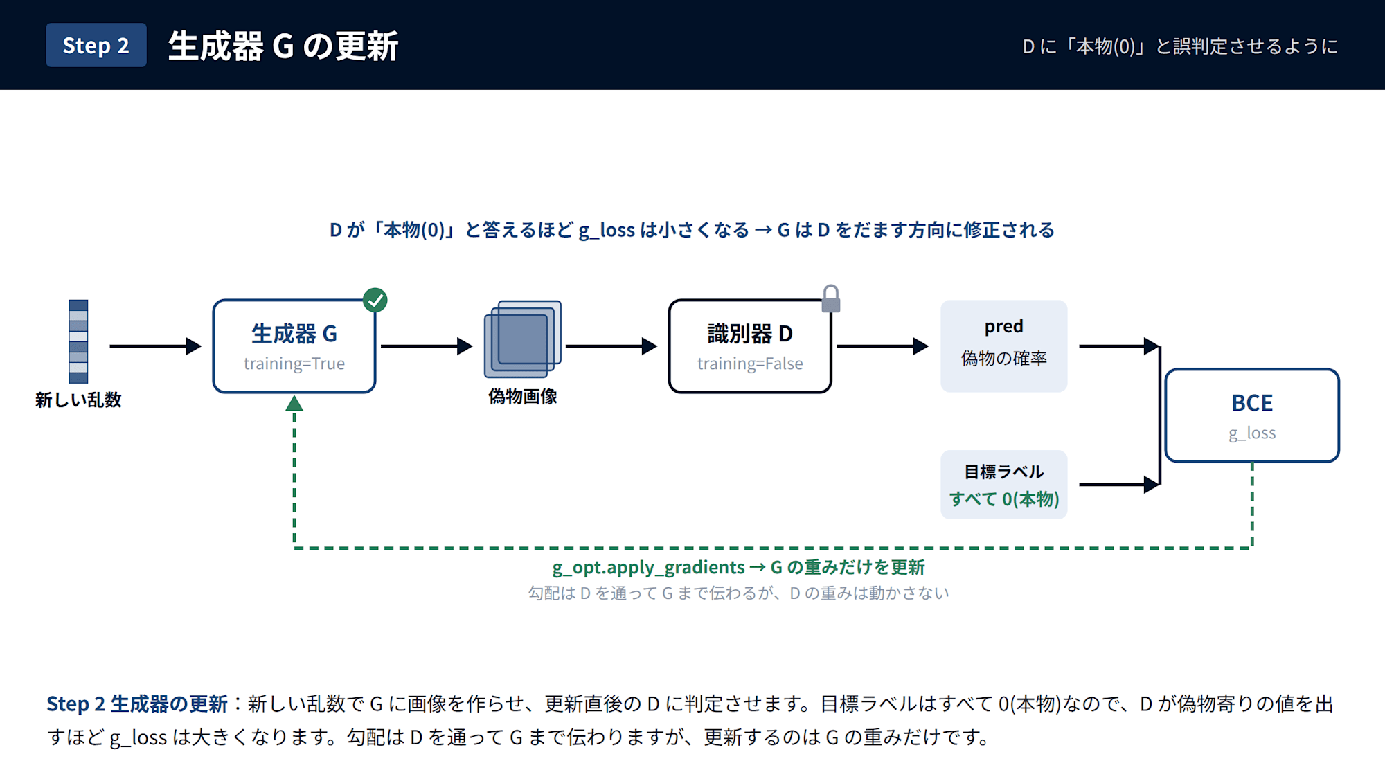
After the discriminator, the generator is updated.
New random noise is used to have the generator create an image, and it is then judged by the discriminator just updated in Step 1.
This time, the discriminator is called with training=False, so Dropout in the discriminator is also disabled.
The target label is "all 0 (real)."
The more fake-leaning the value the discriminator outputs, the larger g_loss becomes, so the generator is corrected in the direction of fooling the discriminator.
As shown by the green dashed line in the figure, the gradient flows back through the discriminator to the generator, but only the generator's weights are updated.
I'd like you to recall — do you remember that the generator has never seen a single real clothing image?
Despite this, the reason the generator becomes able to produce clothing-like images is that it adjusts its weights using the discriminator's judgment — a discriminator that learned from real images — as a guide.
To use an analogy: only the teacher (discriminator) can see the reference painting, and the student (generator) improves their drawing guided only by the teacher's red-pen corrections.
If the teacher doesn't improve, the red-pen feedback becomes inaccurate, and the student won't improve either. Conversely, if the teacher is too strict and marks everything wrong no matter what is drawn, the student won't know what to fix.
The reason I said at the beginning that "the most important thing when running GAN is the power balance between the two models" is precisely because of this relationship.
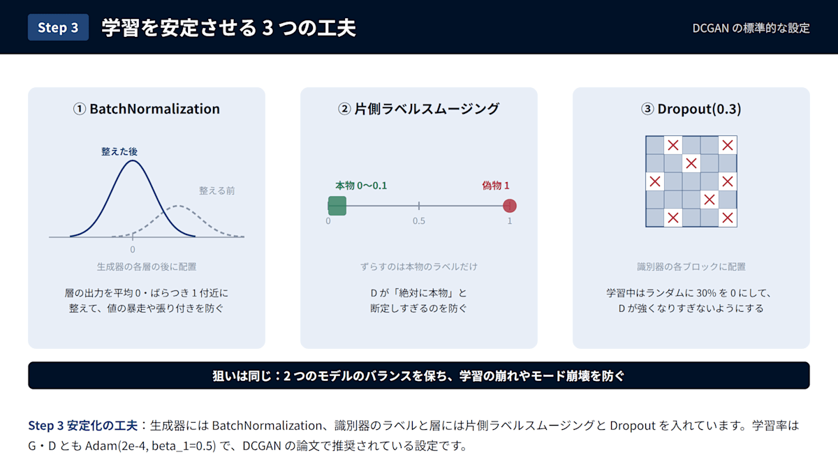
Let me summarize the techniques introduced so far for stabilizing training:
- Insert
BatchNormalizationin each layer of the generator to keep value ranges in order - Label smoothing, where only the real labels are shifted slightly
- Insert
Dropoutin the discriminator to prevent it from becoming too strong
Execution
# ---------------------------------------------------------------- Visualization & Saving
# Fixed random noise for progress monitoring. Since the values are the same every time, you can track how "the same outfit" evolves across epochs.
FIXED_NOISE = tf.random.Generator.from_seed(0).normal((16, NOISE_DIM))

def save_grid(generator, path, noise=None, rows=4, cols=4):
    """Save generated images as a rows x cols grid. If noise is omitted, random noise is used each time."""
    if noise is None:
        noise = tf.random.normal((rows * cols, NOISE_DIM))
    imgs = generator(noise, training=False)
    fig, axes = plt.subplots(rows, cols, figsize=(cols * 2, rows * 2))
    for ax, img in zip(axes.flat, imgs):
        # Fix brightness range to -1~1 (auto-adjustment can make corrupted images appear to have patterns)
        ax.imshow(img[..., 0], cmap="gray", vmin=-1, vmax=1)
        ax.axis("off")
    fig.savefig(path, bbox_inches="tight")
    plt.close(fig)

class Saver(callbacks.Callback):
    """Save checkpoints every few dozen steps and at the end of each epoch. Losses are appended to a CSV."""

    def on_train_batch_end(self, batch, logs=None):
        if (batch + 1) % SAVE_EVERY_STEPS == 0:
            self.model.save_ckpt()

    def on_epoch_end(self, epoch, logs=None):
        save_grid(self.model.g, f"{OUT}/epoch_{epoch + 1:04d}.png", noise=FIXED_NOISE)
        with open(f"{OUT}/loss.csv", "a", newline="") as f:
            csv.writer(f).writerow([epoch + 1, float(logs["d_loss"]), float(logs["g_loss"])])
        self.model.epoch.assign(epoch + 1)
        self.model.save_ckpt()

def plot_loss():
    """Draw a graph from the entire loss.csv (remains continuous even across resumed runs)."""
    if not os.path.exists(f"{OUT}/loss.csv"):
        return
    with open(f"{OUT}/loss.csv") as f:
        rows = [list(map(float, r)) for r in csv.reader(f) if r]
    plt.figure()
    plt.plot([r[0] for r in rows], [r[1] for r in rows], label="d_loss")
    plt.plot([r[0] for r in rows], [r[2] for r in rows], label="g_loss")
    plt.xlabel("epoch")
    plt.legend()
    plt.savefig(f"{OUT}/loss.png")
    plt.close()

# ---------------------------------------------------------------- Execution
if __name__ == "__main__":
    gan = GAN(build_generator(), build_discriminator())
    start = gan.restore()

    # If Ctrl+C or a normal termination signal is received, save before stopping (press Ctrl+C once and wait a few seconds)
    def on_signal(signum, frame):
        print(f"\nsignal {signum}: saving checkpoint...")
        gan.save_ckpt()
        sys.exit(0)

    signal.signal(signal.SIGINT, on_signal)
    signal.signal(signal.SIGTERM, on_signal)

    if start < EPOCHS:
        gan.fit(load_dataset(), initial_epoch=start, epochs=EPOCHS, shuffle=False, callbacks=[Saver()])
    else:
        print(f"already trained {start} epochs")

    plot_loss()
    save_grid(gan.g, f"{OUT}/result.png")
    gan.g.save(f"{OUT}/generator.keras")
    gan.d.save(f"{OUT}/discriminator.keras")
    print(f"done → {OUT}/")
Now it's time to run it.
※ Here, in addition to the training itself, we have set up a mechanism to visually monitor progress and a mechanism for saving checkpoints midway. I wanted a way to keep it running even if I close my PC.
Once training is complete, the loss transition graph (loss.png), the final generated images (result.png), and the generator and discriminator models (.keras) are saved to the output folder.
Execution Results
Training for 20 epochs on a Mac (CPU only) took approximately 4.5 minutes per epoch, for a total of about 1 hour and 35 minutes.
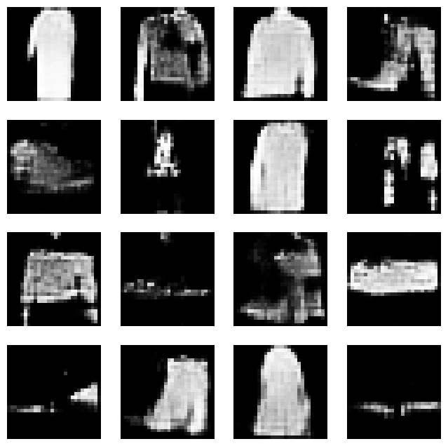
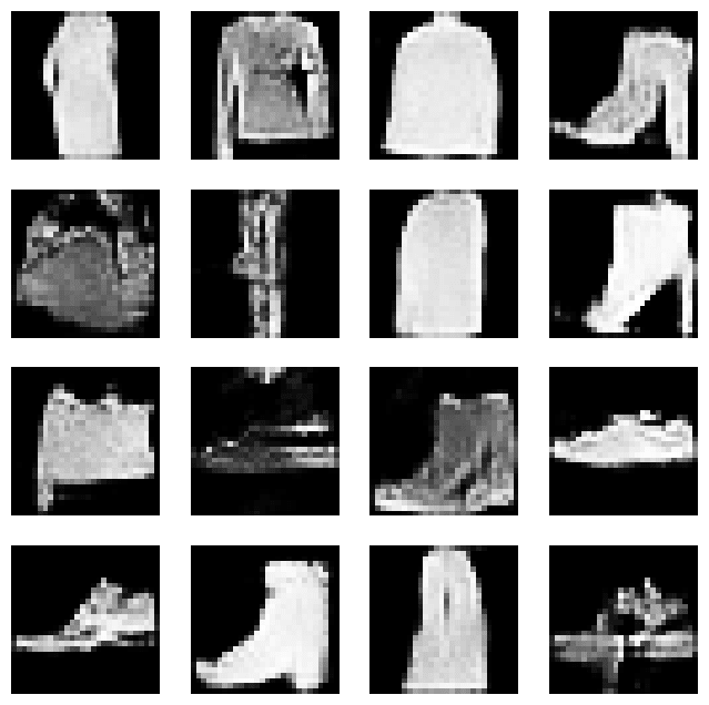
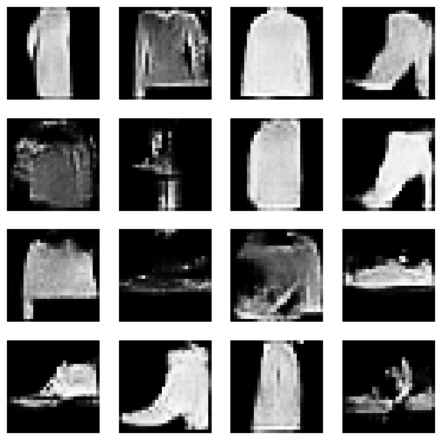
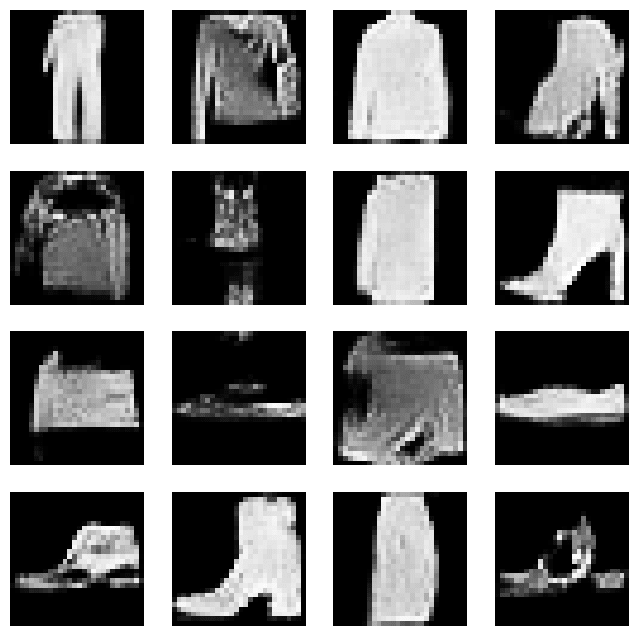
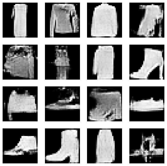
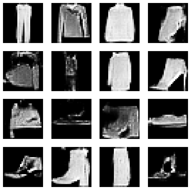
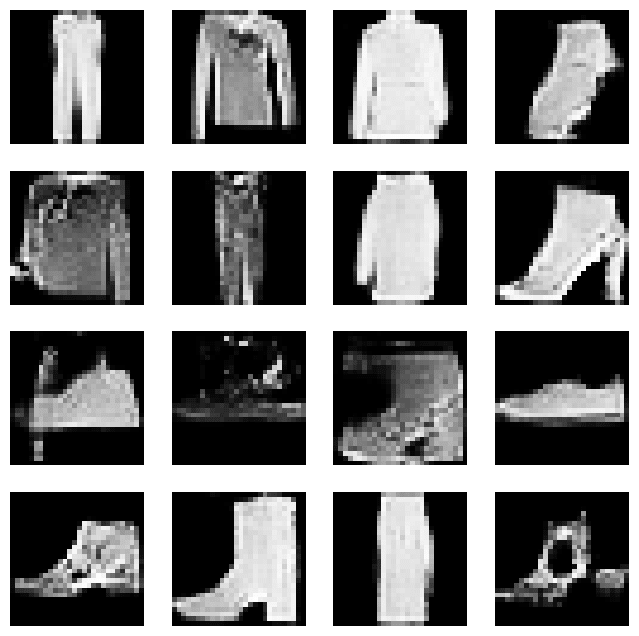
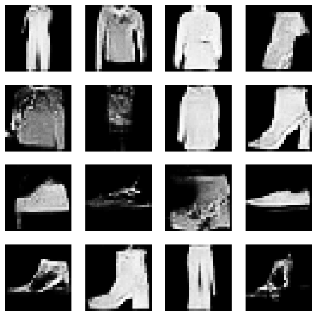
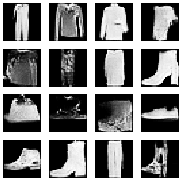
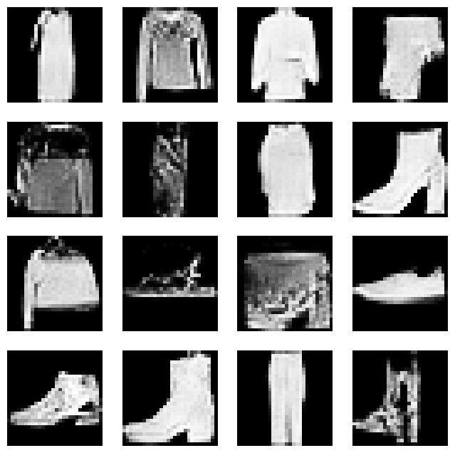
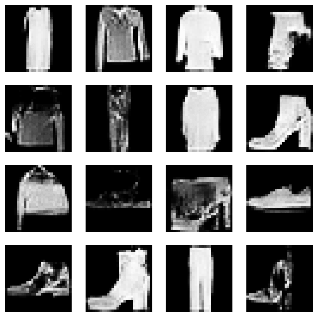
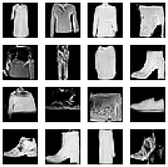
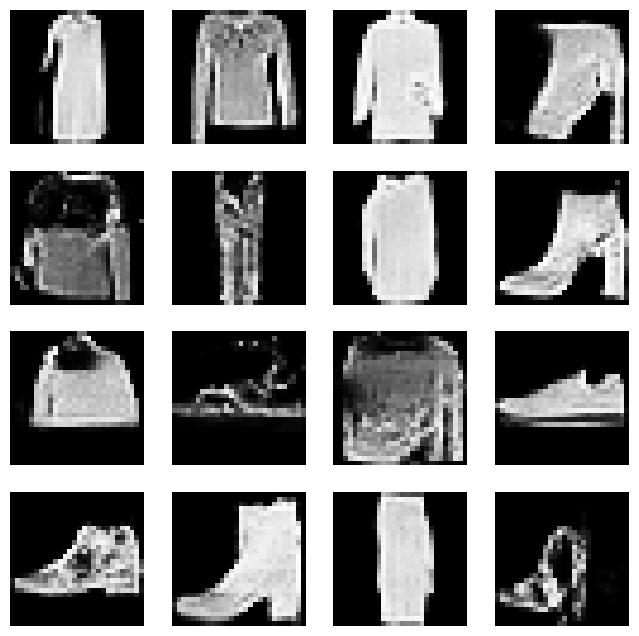
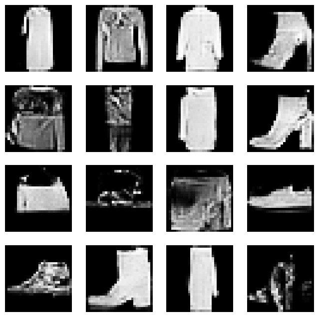
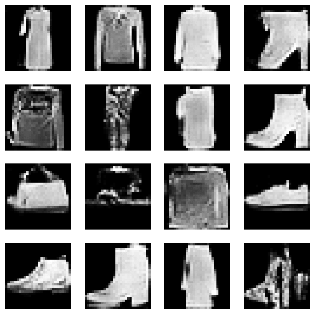
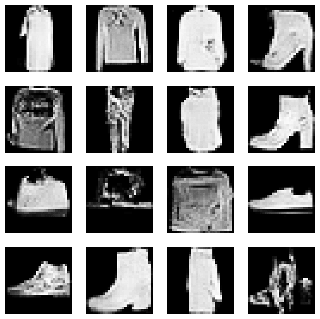
First, let's look at how the images generated from the same 16 random noise vectors changed across epochs.
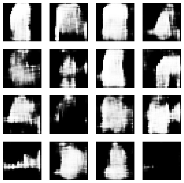
In epoch 1, the output is a blurry white blob — a bit unsettling.
However, each of the 16 images has a different shape, showing that even at this point the model is already trying to produce different outputs for different random inputs.
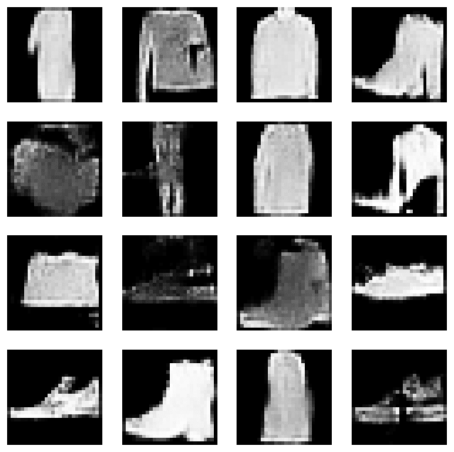
By epoch 3, the images are already recognizable as clothing. You can make out pants, long-sleeved shirts, sneakers, boots, high heels, bags, and dresses.
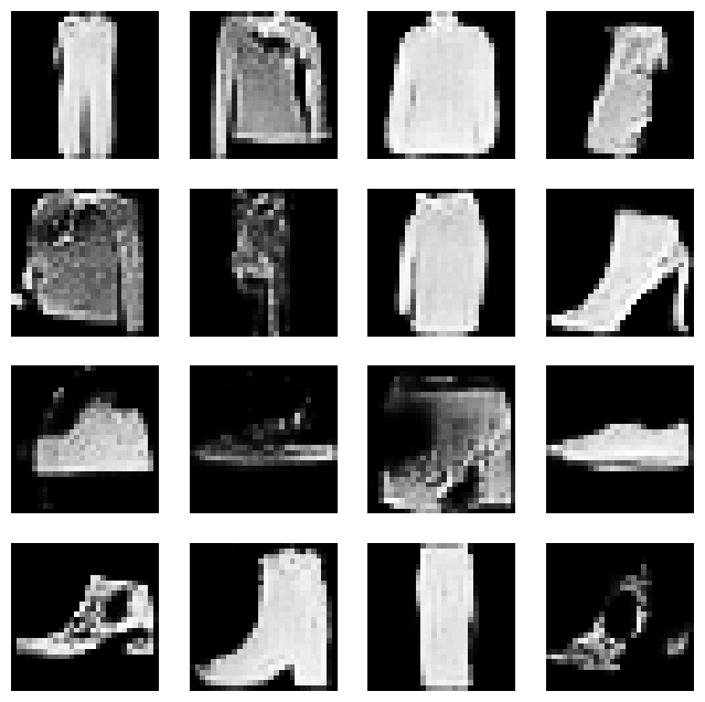
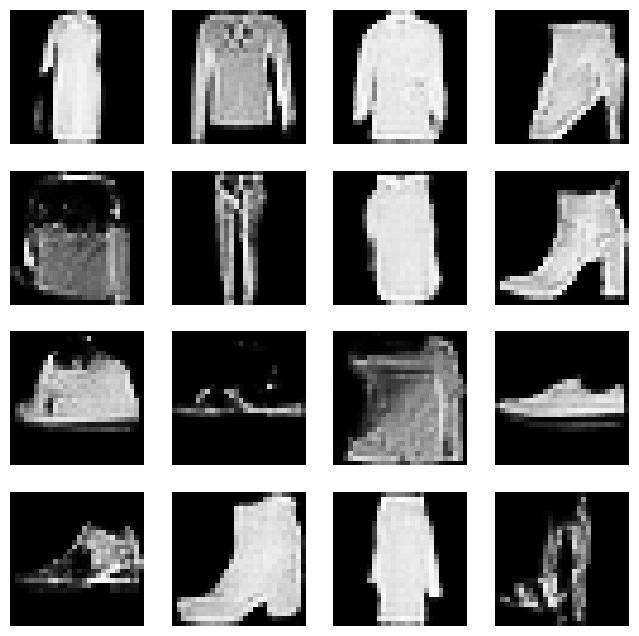
From epoch 9 onward, the types of clothing remain mostly the same, and it appears the model has entered a phase of refining finer details.
By the final epoch 20, the two legs of the pants are clearly separated, and the heels of boots and the outlines of sneakers have become much sharper.
Finally, the image below shows outputs generated by feeding random noise into the trained model each time.
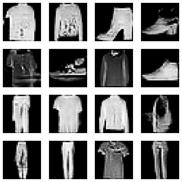
A variety of clothing types are appearing in the output. No "mode collapse" either.
On the other hand... images of detailed shapes like sandals still look noisy, hinting at the limits of this small 28×28 model.
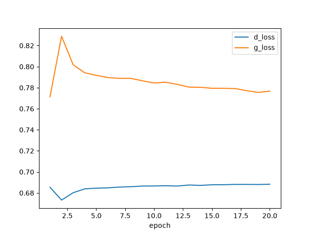
The loss transition shows a slight fluctuation in the first 2–3 epochs, after which it looks very stable.
This means the discriminator can barely distinguish real from fake — the graph confirms the model is approaching the ideal state for a GAN.
Since a GAN involves two models competing against each other, the loss does not continuously decrease toward 0 as it does in typical machine learning.
Conversely, if you want to build an image classification or recognition model, the desirable approach would be to minimize this loss as much as possible.
Summary
In this project, we built a model that generates images of clothing that does not exist in reality using a GAN.
As a result, even on a Mac without a GPU, training for 20 epochs — about 1.5 hours — was enough to generate images where clothing types are distinguishable.
Today's image generation AI is dominated by diffusion models and operates at a much larger scale, but the underlying idea of creating images from random noise and learning to produce plausible images using training data as a reference is the same.
Having run a small model at least once should serve as a good stepping stone when learning about the mechanisms behind larger image generation AIs.
References
- Generative Adversarial Networks(Goodfellow et al., 2014)
- Unsupervised Representation Learning with Deep Convolutional Generative Adversarial Networks(Radford et al., 2015)
- zalandoresearch/fashion-mnist - GitHub
- Deep Convolutional Generative Adversarial Network (DCGAN) - TensorFlow Core
APPENDIX
Below are all the result images from every epoch of the trained model, attached in epoch order.
Looking at them this way, it's fascinating to see how the output gradually evolves from nothing but a blurry haze of random noise into recognizable fashion images!