I tried running and comparing time series foundation models on DGX Spark
This page has been translated by machine translation. View original
Hello, I'm Shigeru Morishige from Classmethod's Manufacturing Business Technology Division.
Starting in the fall of 2025, major updates to time-series foundation models were released in rapid succession. Google's TimesFM 2.5, NVIDIA's NV-Tesseract (currently in evaluation license stage), and AWS's Chronos-2 — three major models from three companies lined up within just two months. Each has slightly different target areas, such as demand forecasting, anomaly detection, and sensor monitoring in manufacturing, and the debate continues over which one comes out on top in benchmarks.
In this article, I benchmark Chronos-2 and TimesFM 2.5, which can be run locally, and introduce NV-Tesseract — which at this point can only be accessed via DGX Cloud NIM — as reading material based on official information and Cognite's case study. The verification environment used is my own DGX Spark.
Positioning and Comparison of the 3 Models
Organizing the three models by developer, distribution format, and intended use case at the ecosystem level gives us the following picture. AWS puts it on SageMaker JumpStart and Bedrock Marketplace, Google puts it on BigQuery's AI.FORECAST, and NVIDIA provides it as a NIM on DGX Cloud — it's interesting how each company's platform strategy is transparently reflected in this.
Placing the major specs side by side makes the commonalities and differences clearly visible.
| Item | Chronos-2 | TimesFM 2.5 | NV-Tesseract |
|---|---|---|---|
| Provider | AWS (Amazon Science) | Google Research | NVIDIA |
| Release | 2025-10-20 | 2025-09 | 2025 (Evaluation license) |
| Architecture | T5 encoder + Group Attention | Decoder-only + quantile head | Transformer (details undisclosed) |
| Parameters | 120M / 28M | 200M | Undisclosed |
| Context Limit | 8,192 | 16,384 | Undisclosed |
| Multivariate Forecasting | Native support | Supported | Supported |
| Anomaly Detection | - (Forecast-focused) | AI.DETECT_ANOMALIES GA |
Native (NV-Tesseract-AD) |
| Fine-Tuning | Publicly available | Publicly available | Via NIM only |
| License | Apache 2.0 | Apache 2.0 | Evaluation license |
| Availability | HF / GitHub | HF / JAX version available | DGX Cloud NIM only |
| Commercial Use | Yes | Yes | Conditional during evaluation period |
While both Chronos-2 and TimesFM 2.5 are Apache 2.0 and can run locally, NV-Tesseract is in the evaluation license stage and can only be accessed via DGX Cloud NIM — a notable difference in availability. No announcement has been made regarding the general release date as of this time. (As of May 2026)
Verification Environment
Both models work entirely through Python library calls. Since dependency versions conflict with each other, I set up separate uv venv environments.
| Item | Value |
|---|---|
| Hardware | DGX Spark (NVIDIA GB10, aarch64, 128GB UMA) |
| OS / Driver | Ubuntu 24.04 / NVIDIA driver 580.142 |
| Python | 3.13.13 |
| PyTorch | 2.12.0+cu130 (common to both venvs) |
| For Chronos-2 | chronos-forecasting==2.2.2, transformers==4.57.6 |
| For TimesFM 2.5 | timesfm==2.0.0 (git head d720daa6), safetensors==0.7.0 |
Trying Chronos-2
Just install chronos-forecasting>=2.1.0 (2.1.0 and later include bug fixes for past-value covariates) via pip. For PyTorch, I explicitly specify the cu130 wheel index for ARM64 + Blackwell GB10.
uv pip install --index-url https://download.pytorch.org/whl/cu130 \
  --extra-index-url https://pypi.org/simple/ torch
uv pip install "chronos-forecasting>=2.1.0"
The minimal sample looks like this. It goes straight through from BaseChronosPipeline.from_pretrained to predict_quantiles, returning 21 quantiles in a single inference after loading.
import numpy as np
import torch
from chronos import BaseChronosPipeline

pipeline = BaseChronosPipeline.from_pretrained(
    "amazon/chronos-2", device_map="cuda", dtype=torch.bfloat16
)
# Input is a 3D tensor of shape (n_series, n_variates, history_length)
context = torch.tensor(np.arange(512, dtype=np.float32)[None, None, :])
quantiles_list, mean_list = pipeline.predict_quantiles(
    context, prediction_length=96, quantile_levels=[0.1, 0.5, 0.9]
)
print(quantiles_list[0].shape)  # torch.Size([1, 96, 3])
One thing to be careful about is that chronos-forecasting>=2.2 has completely revamped the argument names, input shape, and return values of predict_quantiles, so copy-pasting from older articles or official examples is unlikely to work without modification.
Trying TimesFM 2.5
The one thing to watch out for with TimesFM 2.5 is that the timesfm==1.3.0 distributed on PyPI does not yet include the TimesFM 2.5 API. The Hugging Face model card also explicitly states "pip install from PyPI coming soon. At this point, please git clone," so for now there is no choice but to install from GitHub HEAD. Since we install with --no-deps, we specify safetensors separately.
uv pip install --index-url https://download.pytorch.org/whl/cu130 \
  --extra-index-url https://pypi.org/simple/ torch safetensors
uv pip install --force-reinstall --no-deps \
  "timesfm @ git+https://github.com/google-research/timesfm.git"
Here is the minimal sample. The pattern is to define the context and horizon limits using ForecastConfig and compile, then pass the actual forecast length to forecast.
import numpy as np
import timesfm

model = timesfm.TimesFM_2p5_200M_torch.from_pretrained(
    "google/timesfm-2.5-200m-pytorch"
)
model.compile(timesfm.ForecastConfig(
    max_context=2048, max_horizon=256,
    normalize_inputs=True, use_continuous_quantile_head=True,
    fix_quantile_crossing=True,
))
point_forecast, quantile_forecast = model.forecast(
    horizon=96, inputs=[np.arange(512, dtype=np.float32)],
)
print(point_forecast.shape)  # (1, 96)
Benchmark Results
From here, I evaluate the three models on ETTh1 (an electricity dataset) across three axes: latency, accuracy, and memory efficiency.
I used the OT column (oil temperature) from ETTh1 (Electricity Transformer Temperature, Hourly, 7 variables, 17,420 rows). This is a dataset where a Chinese electricity company monitored distribution transformers for two years (July 2016 to July 2018), aiming to predict signs of overheating accidents from the transformer's internal oil temperature (OT) and 6 types of load variables (high/medium/low active/reactive power). Its structure is close to equipment monitoring data in manufacturing, and since the Informer paper (AAAI 2021 Best Paper), it has been used as a standard benchmark for time-series forecasting.
Evaluation was performed by taking 64 rolling-window splits from the end with step=24. Metrics are MASE (Mean Absolute Scaled Error) and RMSE, inference latency is the warm median with cold/warm separated, and peak GPU memory is obtained using torch.cuda.max_memory_allocated().
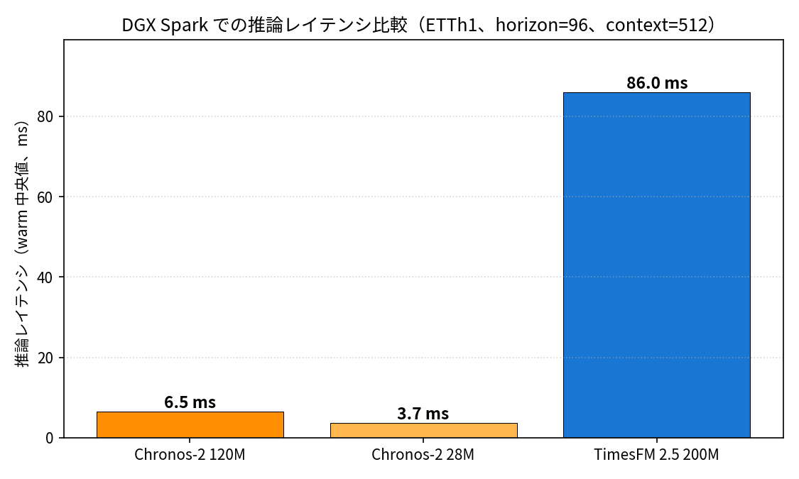
Short-term Forecasting (horizon=96, context=512)
| Model | Warm Median | Warm p95 | Peak GPU mem | MASE | RMSE |
|---|---|---|---|---|---|
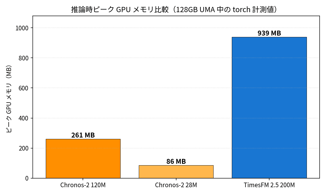
| Chronos-2 120M | 6.5 ms | 6.7 ms | 0.255 GB | 1.149 | 2.228 |
| Chronos-2 28M | 3.7 ms | 3.9 ms | 0.084 GB | 1.154 | 2.263 |
| TimesFM 2.5 200M | 86.0 ms | 89.3 ms | 0.917 GB | 1.106 | 2.169 |
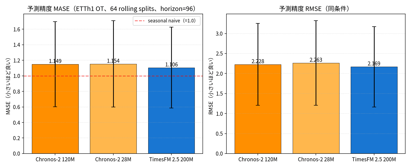
In terms of accuracy, TimesFM 2.5 achieves the best MASE and RMSE, but all three models only marginally outperform seasonal naive (MASE=1.0, which simply returns the value from 24 hours ago). Since ETTh1 OT has a strong daily periodicity, seasonal baseline is a reasonably tough opponent even for zero-shot foundation models.
The latency gap is quite striking: Chronos-2 28M (3.7ms) and Chronos-2 120M (6.5ms) are 13 to 23 times faster than TimesFM 2.5 200M (86ms). This directly reflects the architectural difference between Chronos-2, which outputs all quantiles in a single forward pass with an encoder, and TimesFM 2.5, which generates autoregressively with a decoder.
In terms of GPU memory, the 28M model uses 1/3 of the 120M model and 1/11 of TimesFM 2.5, while achieving nearly equivalent accuracy.
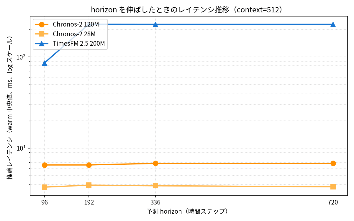
What Happens When You Extend the Horizon
I extended the forecast target from 96 hours (4 days) to 720 hours (30 days) to see how latency and accuracy change.
| horizon | Chronos-2 120M | Chronos-2 28M | TimesFM 2.5 200M |
|---|---|---|---|
| 96 | 6.5 ms / MASE 1.149 | 3.7 ms / MASE 1.154 | 86 ms / MASE 1.106 |
| 192 | 6.7 ms / 1.196 | 3.8 ms / 1.221 | 229 ms / 1.241 |
| 336 | 6.8 ms / 1.259 | 3.9 ms / 1.330 | 228 ms / 1.214 |
| 720 | 6.8 ms / 1.453 | 3.8 ms / 1.543 | 228 ms / 1.411 |
Chronos-2's latency is almost the same between horizon=96 and horizon=720 (6.5ms → 6.8ms), which is quietly impressive. TimesFM 2.5 increased 2.7x from h=96 to h=192, then plateaued as the internal horizon_len hit a ceiling.
In terms of accuracy, all models naturally degrade as the horizon extends, but TimesFM 2.5 still slightly outperforms Chronos-2 120M (1.453) at h=720 with a MASE of 1.411. Maintaining its accuracy advantage even in long-horizon forecasting is a strength of TimesFM 2.5.
TimesFM 2.5 Shows Dramatic Accuracy Improvement When Context Is Extended
Since TimesFM 2.5 promotes its "16K context," whether accuracy truly improves when context is extended was a point I wanted to verify. Since Chronos-2 has a context limit of 8,192, this evaluation was done for TimesFM 2.5 alone.
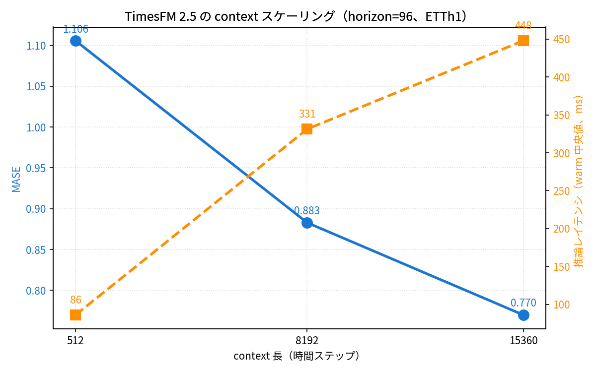
| context | Warm Median | Peak GPU | MASE | vs c=512 |
|---|---|---|---|---|
| 512 | 86.0 ms | 0.917 GB | 1.106 | baseline |
| 8,192 | 331.2 ms | 0.993 GB | 0.883 | 20% improvement |
| 15,360 | 447.8 ms | 1.074 GB | 0.770 | 30% improvement |
At c=15,360, MASE is 0.770, which is 23% better than seasonal naive. The effect of the "16K context" clearly shows up in the numbers, reinforcing the impression that this is a model where long context is genuinely effective. One thing to note is that you cannot use the full 16,384 model limit for context — there is an architectural constraint that max_context + max_horizon ≤ 16384, so if you reserve horizon=1024, the practical context limit is up to 15,360.
Multivariate Forecasting
Since ETTh1 has 6 power load columns besides OT — HUFL / HULL / MUFL / MULL / LUFL / LULL — I tested how the OT-only accuracy changes when predicting all 7 variables simultaneously with Chronos-2 in multivariate mode.
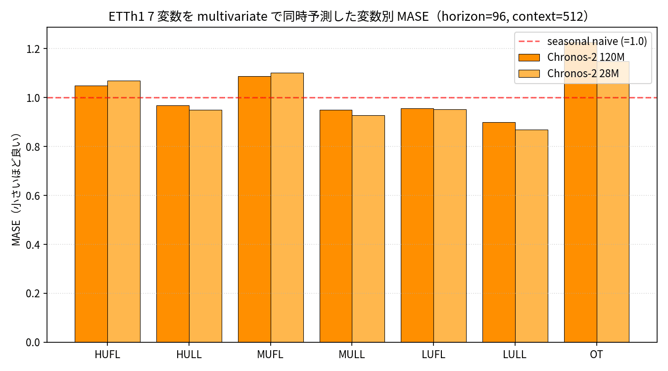
As a result, looking at OT accuracy with Chronos-2 120M, it worsened by 7% from the univariate MASE of 1.149 to 1.226 in the multivariate setting. On the other hand, the other 6 variables were forecasted well with MASE ranging from 0.87 to 1.09, with LULL in particular achieving 0.90, outperforming seasonal naive by 10%.
This likely reflects a phenomenon commonly seen in machine learning: "mixing in covariates that are weakly correlated with the target can be counterproductive." Trying the same thing with Chronos-2 28M, the OT MASE remained nearly unchanged at 1.149, and this version seems well-suited for dashboard use cases where all metrics are returned in a single forward pass.
Is the Ranking Maintained in Other Domains?
To see whether the ranking obtained on ETTh1 (electricity data) holds in other domains, I ran the same conditions on the T column (room temperature in Rome) from the UCI Air Quality dataset.
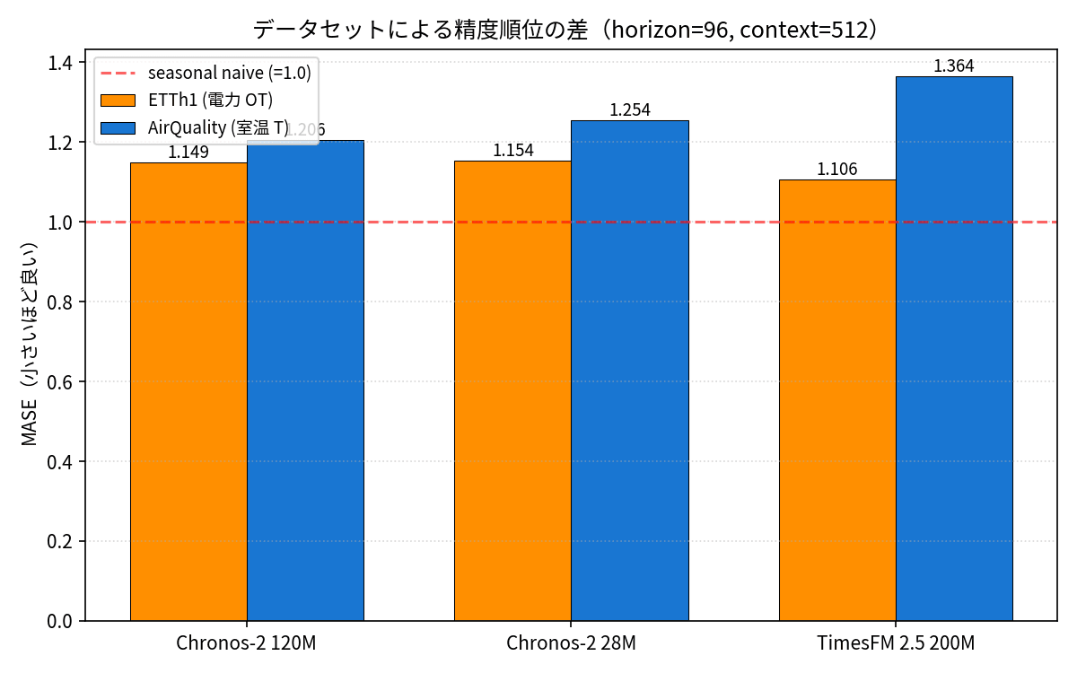
| Dataset | 1st | 2nd | 3rd |
|---|---|---|---|
| ETTh1 (Electricity OT) | TimesFM 2.5 (1.106) | Chronos-2 120M (1.149) | Chronos-2 28M (1.154) |
| AirQuality (Room Temperature T) | Chronos-2 120M (1.206) | Chronos-2 28M (1.254) | TimesFM 2.5 (1.364) |
The ranking reversed. AirQuality has more noise as a time series than ETTh1, and since it lacks as strong a daily periodicity (there is a day/night difference but also large seasonal variation), it seems that with short context (c=512), the long-context strength of TimesFM 2.5 is not being utilized. This is a result showing that "TimesFM 2.5 is not always the best," reinforcing the importance of actually comparing models in the target production domain.
Anomaly Detection Simulation
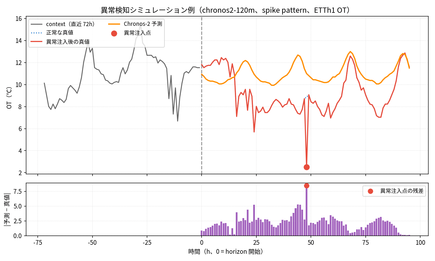
Hearing that NV-Tesseract is strong at anomaly detection makes you wonder how useful prediction-based anomaly detection with Chronos-2 / TimesFM 2.5 actually is. I artificially injected three types of anomalies — spikes, level shifts, and noise bursts — into the ETTh1 test segment and calculated the per-step ROC AUC using the absolute value of the prediction residual as the anomaly score.
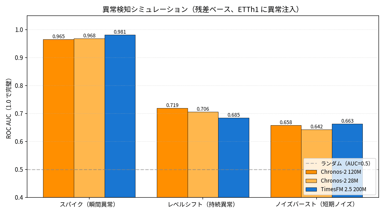
| Pattern | Chronos-2 120M | Chronos-2 28M | TimesFM 2.5 200M |
|---|---|---|---|
| Spike (instantaneous anomaly) | 0.965 | 0.968 | 0.981 |
| Level Shift (persistent anomaly) | 0.719 | 0.706 | 0.685 |
| Noise Burst (short-term) | 0.658 | 0.642 | 0.663 |
All three models achieve AUC above 0.96 for spikes, meaning instantaneous outliers can be caught almost reliably. The chart below shows a qualitative example — prediction residuals spike only at the injected spike locations (red circles), which is visually clear.
Level shifts show moderate performance with AUC of 0.69 to 0.72 — a level where gradual drift-type anomalies in equipment can be detected to a reasonable degree. Noise bursts are lower at AUC 0.64 to 0.67, suggesting that short-term high-frequency noise is likely to be missed by prediction-based FM alone. A dedicated anomaly detection model like NV-Tesseract should excel here, and I look forward to comparing them again after its release.
NV-Tesseract
According to the official NVIDIA Developer Blog (New NVIDIA NV-Tesseract Time-Series Models and Advancing Anomaly Detection for Industry Applications), NV-Tesseract is a Transformer-based model supporting three tasks: forecasting, anomaly detection, and classification. In particular, the anomaly detection component (NV-Tesseract-AD) appears to be designed for detecting subtle outliers in industrial sensors using a mechanism called segmented / multi-scale adaptive thresholding.
An impressive real manufacturing case study is the partnership with Cognite announced on the first day of GTC 2026 (March 16, 2026). A case study has been published in which state prediction from water level sensors in a reaction tank at Celanese's chemical plant in Clear Lake, Texas is running via NV-Tesseract NIM. The challenge on Celanese's side was that "every time manual sampling occurred, conventional prediction models would suffer from bias jumps (step changes in bias) that would break continuous operation," and the aim is to bridge this gap with NV-Tesseract's real-time prediction.
What's interesting about the delivery model is that it connects NV-Tesseract NIM to Cognite's Industrial Knowledge Graph (a graph database of equipment, sensors, and operational knowledge), providing data context and model together as a package. The target sectors are not limited to chemicals but extend to energy, manufacturing, power and renewables, and heavy industry — giving a sense of a direction where an OT data platform intermediary serves as the gateway for optimization across entire industrial lines. Combined with video-based foundation models like VSS and Cosmos, there seems to be a path toward factory visualization along both "sensor time series + video" axes.
There is currently no announced timeline for when it will be runnable on local DGX Spark or Jetson, but it's something to look forward to.
Ecosystem and Operational Comparison
Why did the benchmark results in Section 6 turn out the way they did? Looking at the internal architecture of the three models side by side, it becomes clear that differences in design philosophy directly translate into differences in operational characteristics.
Chronos-2 outputs the entire horizon in a single forward pass with encoder + quantile head, so latency doesn't scale much with horizon length. TimesFM 2.5 autoregressively generates patch units with a decoder, so latency increases as the horizon grows, but in return it can take advantage of long context — that's the design trade-off.
Recommendations by use case would be something like the following.
| Intended Use | Likely Best Choice |
|---|---|
| Demand forecasting centered on AWS (rich covariates) | Chronos-2 + SageMaker JumpStart / Bedrock Marketplace |
| One-shot SQL forecasting on a GoogleCloud data lake | TimesFM 2.5 + BigQuery AI.FORECAST |
| IoT sensor anomaly detection (high accuracy requirements) | NV-Tesseract |
| Lightweight operation closer to the edge | Chronos-2 28M |
| Long-horizon trend forecasting (thousands of steps) | TimesFM 2.5 (long context mode) |
| High-volume parallel short-term forecasting | Chronos-2 120M |
| Probabilistic forecasting in finance, etc. | Chronos-2 |
Considerations for Real-World Project Applications
In a project I'm currently involved with, I'm thinking about using real-time data acquired from PLCs (industrial controllers that manage sensors and setpoints on the factory floor) fed into time-series models to continuously judge "whether the current operating conditions are likely to produce normal products" and "whether setpoint changes show signs of heading toward failure." By passing setpoints as future covariates, you can forecast future quality metrics, and by monitoring prediction residuals, you can generate anomaly scores as well. The benchmark in this article shows that Chronos-2 28M at 3.7ms warm latency easily fits within PLC scan cycles (100ms to 1 second), making real-time integration in an edge-adjacent configuration realistically feasible. The Cognite × Celanese case study mentioned earlier follows exactly the same pattern, implementing this by connecting an OT platform with NIM. I plan to cover the technical verification of feeding actual PLC data in a separate article.
Implementation Pitfalls to Watch Out For
Here are just two points where the transitional state of the libraries — not the time-series models themselves — tends to cause issues.
The predict_quantiles API in Chronos-2 was completely revamped in the 2.2.x series, so copy-pasting from older articles or official examples will not work as-is. The argument is inputs=tensor, the input must be 3-dimensional (n_series, n_variates, history_length) (even for univariate: tensor[None, None, :]), and the return value is tuple[list[Tensor], list[Tensor]] where quantiles_list[0] has shape (n_variates, horizon, num_quantiles).
The practical context limit for TimesFM 2.5 is up to 15,360. There is an architectural constraint that max_context + max_horizon ≤ 16384, so if you reserve horizon=1024, context can only go up to 15,360. The long context verification in this article was also measured at c=15,360.
Summary
In this article, I organized the major updates to time-series foundation models that have been rolling out since fall 2025, benchmarked AWS Chronos-2 and Google TimesFM 2.5 on actual hardware, and introduced NV-Tesseract based on official information and the Cognite case study.
To put it simply, the division looks like: Chronos-2 for latency-critical high-volume parallel processing, TimesFM 2.5 for leveraging long context to maximize accuracy, and NV-Tesseract for dedicated anomaly detection in manufacturing settings. Chronos-2 28M is lightweight in both memory and inference time while achieving nearly the same accuracy as the 120M model — making it an interesting option for deployment in edge-adjacent locations.
Reference Links
Chronos-2
- Amazon Science Blog - Introducing Chronos-2
- GitHub - amazon-science/chronos-forecasting
- arXiv 2510.15821 - Chronos-2: From Univariate to Universal Forecasting
TimesFM 2.5
- HuggingFace - google/timesfm-2.5-200m-pytorch
- GitHub - google-research/timesfm
- BigQuery AI.FORECAST documentation
NV-Tesseract
- NVIDIA Developer Blog - NV-Tesseract Time-Series Models
- NVIDIA Developer Blog - NV-Tesseract-AD for Industry Applications
- Cognite × NVIDIA Partnership