
Hugging Faceを使って事前学習モデルを日本語の感情分析用にファインチューニングしてみた
この記事は公開されてから1年以上経過しています。情報が古い可能性がありますので、ご注意ください。
こんちには。
データアナリティクス事業本部 機械学習チームの中村です。
最近以下の書籍を読んでいます。
こちらの書籍はHugging Faceにおけるライブラリ(Transformersなど)の使用方法について、ライブラリの作者自身が解説した本となっています。 様々なタスクにおける、Hugging Faceのライブラリの使用方法の他、Transformerの進化の歴史や、TransformerのアーキテクチャをゼロからPyTochで実装する箇所もあり、 結構濃い内容でオススメです。
現在まだ途中までしか読めていませんが、読んだ内容を日本語タスクでも試してみたいということで、 本記事では日本語を題材にした、テキスト分類の1つである感情分析をやってみたいと思います。
Hugging Faceの概要
Hugging Faceは主に自然言語処理を扱えるエコシステム全体を提供しています。
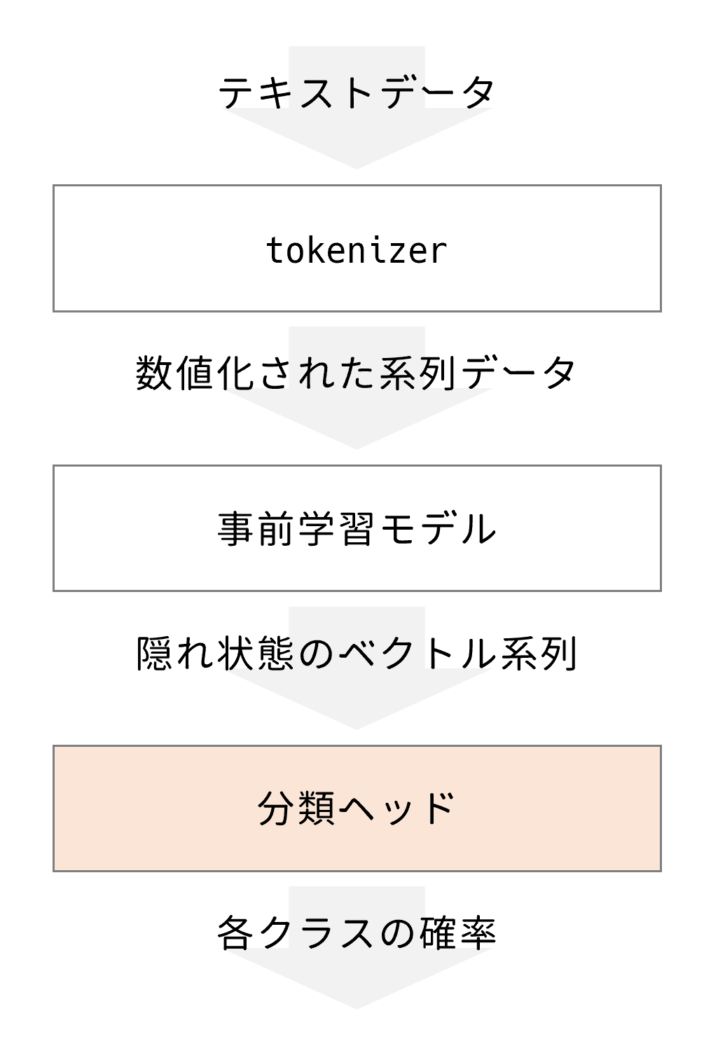
実際に使用する際は以下のようなフローで進めていきます。

各箇所で必要な処理は、transformersやdatasetsなどのライブラリとして提供されています。 またデータセットやモデル(トークナイザ)もHugging Faceのページで検索して必要なものを見つけることが可能です。
今回もこの手順に沿って進めていきます。
やってみた
実行環境
今回はGoogle Colaboratory環境で実行しました。
ハードウェアなどの情報は以下の通りです。
- GPU: Tesla P100 (GPUメモリ16GB搭載)
- CUDA: 11.1
- メモリ: 26GB
主なライブラリのバージョンは以下となります。
- transformers: 4.22.1
- datasets: 2.4.0
インストール
transformersとdatasetsをインストールします。
!pip install transformers
!pip install datasets
データセットの検索
使用するデータセットをまず探す必要があります。
データセットはHugging Faceのページに準備されており、以下から検索が可能です。
今回は以下のデータセットのうち、日本語のサブセットを使用します。
データセットの取得
以下を実行しデータセットを取得します。
from datasets import load_dataset

dataset = load_dataset("tyqiangz/multilingual-sentiments", "japanese")
データセットの確認
取得したデータセットの中身を見てみましょう。
dataset
DatasetDict({
    train: Dataset({
        features: ['text', 'source', 'label'],
        num_rows: 120000
    })
    validation: Dataset({
        features: ['text', 'source', 'label'],
        num_rows: 3000
    })
    test: Dataset({
        features: ['text', 'source', 'label'],
        num_rows: 3000
    })
})
データセットはこのようにtrain, validation, testに分かれています。
それぞれが、['text', 'source', 'label']といった情報を持っていることも分かります。
取得したデータセットは以下のようにフォーマットを設定することで、データフレームとして扱うことも可能です。
dataset.set_format(type="pandas")
train_df = dataset["train"][:]
train_df.head(5)
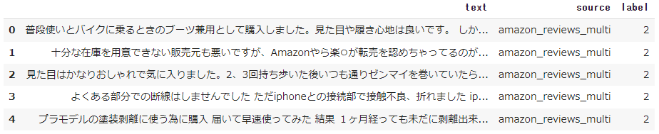
どうやらamazonのレビューデータが元になって、そちらに対してラベルが付与されているようです。
データを理解する上では、データフレームで扱える部分は便利ですね。
sourceとlabelの内訳を見てみましょう。
train_df.value_counts(["source", "label"])
source                label
amazon_reviews_multi  0        40000
                      1        40000
                      2        40000
dtype: int64
sourceは1種類の値しか取らず、labelは3種類であることが分かります。
各ラベルの意味については、featuresを見れば分かるようになっています。
featuresは、各列の値についての詳細が記載してあります。
dataset["train"].features
{'text': Value(dtype='string', id=None),
 'source': Value(dtype='string', id=None),
 'label': ClassLabel(num_classes=3, names=['positive', 'neutral', 'negative'], id=None)}
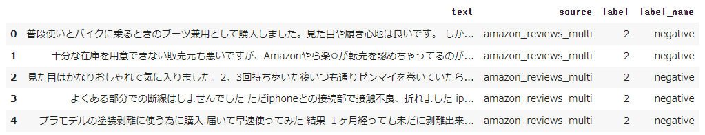
このように、labelはClassLabelクラスとなっており、0,1,2がそれぞれ'positive','neutral','negative'に割り当てられていることが分かります。
ClassLabelクラスには、int2strというメソッドがあり、これでラベル名に変換することが可能です。
def label_int2str(x):
	return dataset["train"].features["label"].int2str(x)

train_df["label_name"] = train_df["label"].apply(label_int2str)
train_df.head()
最後に、データフレームにしていたフォーマットを元に戻しておきます。
dataset.reset_format()
モデルの検索
データをトークナイザで処理する前に、使用する事前学習モデルを決める必要があります。理由としては、通常事前学習モデルを作成した時と同じトークナイザを使用する必要があるためと考えられます。
モデルの検索もHugging Faceのページに準備されており、以下から検索が可能です。
この中で、BERTの日本語版を探し、その中が比較的ダウンロード数の多い以下を使用することにします。
他にも様々な事前学習モデルがありますが、後述するトークナイザの精度などを確認し、問題が無さそうなものを選択しました。
トークナイザの動作確認
トークナイザ利用前に以降でライブラリが不足しているというエラーが出るため、以下をインストールしました。
!pip install fugashi
!pip install ipadic
その後、トークナイザをAutoTokenizerで呼び出します。
from transformers import AutoTokenizer

model_ckpt = "cl-tohoku/bert-base-japanese-whole-word-masking"
tokenizer = AutoTokenizer.from_pretrained(model_ckpt)
トークナイザを動かしてみましょう。
とりあえずサンプルのテキストを自身の過去のブログ記事から拝借してきました。
sample_text = "\
機械学習のコア部分のロジックを、定型的な実装部分から切り離して\
定義できるようなインターフェースに工夫されています。 \
そのためユーザーは、機械学習のコア部分のロジックの検討に\
集中することができます。\
"
トークナイザの結果は以下で得られます。
sample_text_encoded = tokenizer(sample_text)
print(sample_text_encoded)
{'input_ids': [2, 2943, 4293, 5, 6759, 972, 5, 138, 17394, 11, 6, 23398, 81, 18, 6561,
972, 40, 24547, 16, 2279, 392, 124, 18, 23953, 7, 9909, 26, 20, 16, 21, 2610, 8, 59,
82, 4502, 9, 6, 2943, 4293, 5, 6759, 972, 5, 138, 17394, 5, 3249, 7, 4155, 34, 45, 14,
203, 2610, 8, 3], 'token_type_ids': [0, 0, 0, 0, 0, 0, 0, 0, 0, 0, 0, 0, 0, 0, 0, 0,
0, 0, 0, 0, 0, 0, 0, 0, 0, 0, 0, 0, 0, 0, 0, 0, 0, 0, 0, 0, 0, 0, 0, 0, 0, 0, 0, 0, 0,
0, 0, 0, 0, 0, 0, 0, 0, 0, 0, 0], 'attention_mask': [1, 1, 1, 1, 1, 1, 1, 1, 1, 1, 1,
1, 1, 1, 1, 1, 1, 1, 1, 1, 1, 1, 1, 1, 1, 1, 1, 1, 1, 1, 1, 1, 1, 1, 1, 1, 1, 1, 1, 1,
1, 1, 1, 1, 1, 1, 1, 1, 1, 1, 1, 1, 1, 1, 1, 1]}
結果はこのように、input_idsとattention_maskが含まれます。
input_idsは数字にエンコードされたトークンで、attention_maskは後段のモデルで有効なトークンかどうかを判別するためのマスクです。
無効なトークン(例えば、[PAD]など)に対しては、attention_maskを0として処理します。
トークナイザの結果は数字にエンコードされているため、トークン文字列を得るには、convert_ids_to_tokensを用います。
tokens = tokenizer.convert_ids_to_tokens(sample_text_encoded.input_ids)
print(tokens)
['[CLS]', '機械', '学習', 'の', 'コア', '部分', 'の', 'ロ', '##ジック', 'を', '、',
'定型', '的', 'な', '実装', '部分', 'から', '切り離し', 'て', '定義', 'できる',
'よう', 'な', 'インターフェース', 'に', '工夫', 'さ', 'れ', 'て', 'い', 'ます', '。',
 'その', 'ため', 'ユーザー', 'は', '、', '機械', '学習', 'の', 'コア', '部分', 'の',
 'ロ', '##ジック', 'の', '検討', 'に', '集中', 'する', 'こと', 'が', 'でき', 'ます',
 '。', '[SEP]']
結果がこのように得られます。
先頭に##が付加されているものは、サブワード分割されているものです。
また、系列の開始が[CLS]、系列の終了(実際は複数系列の切れ目)が[SEP]という特殊なトークンとなっています。
トークナイザについては以下にも説明があります。
The texts are first tokenized by MeCab morphological parser with the IPA dictionary and then split into subwords by the WordPiece algorithm. The vocabulary size is 32000.
トークン化にIPA辞書を使ったMecabが使用され、サブワード分割にはWordPieceアルゴリズムが使われているようです。
その他、文字列を再構成するには、convert_tokens_to_stringを用います。
decode_text = tokenizer.convert_tokens_to_string(tokens)
print(decode_text)
[CLS] 機械 学習 の コア 部分 の ロジック を 、 定型 的 な 実装 部分 から 切り離し て
定義 できる よう な インターフェース に 工夫 さ れ て い ます 。 その ため ユーザー
は 、 機械 学習 の コア 部分 の ロジック の 検討 に 集中 する こと が でき ます 。
[SEP]
データセット全体のトークン化
データセット全体に処理を適用するには、バッチ単位で処理する関数を定義し、mapを使って実施します。
padding=Trueでバッチ内の最も長い系列長に合うようpaddingする処理を有効にします。truncation=Trueで、後段のモデルが対応する最大コンテキストサイズ以上を切り捨てます。
def tokenize(batch):
    return tokenizer(batch["text"], padding=True, truncation=True)
参考までにモデルが対応する最大コンテキストサイズは、以下で確認ができます。
tokenizer.model_max_length
512
これをデータセット全体に適用します。
batched=Trueによりバッチ化され、batch_size=Noneにより全体が1バッチとなります。
dataset_encoded = dataset.map(tokenize, batched=True, batch_size=None)
結果を以下で確認します。
dataset_encoded
DatasetDict({
    train: Dataset({
        features: ['text', 'source', 'label', 'input_ids', 'token_type_ids', 'attention_mask'],
        num_rows: 120000
    })
    validation: Dataset({
        features: ['text', 'source', 'label', 'input_ids', 'token_type_ids', 'attention_mask'],
        num_rows: 3000
    })
    test: Dataset({
        features: ['text', 'source', 'label', 'input_ids', 'token_type_ids', 'attention_mask'],
        num_rows: 3000
    })
})
これだけで、データセット全体に適用され、カラムが追加されていることが分かります。
token_types_idは今回使用しませんが、複数の系列がある場合に使用されます。(詳細は下記を参照)
サンプル単位で結果を確認したい場合は、データフレームなどを使用します。
import pandas as pd
sample_encoded = dataset_encoded["train"][0]
pd.DataFrame(
    [sample_encoded["input_ids"]
     , sample_encoded["attention_mask"]
     , tokenizer.convert_ids_to_tokens(sample_encoded["input_ids"])],
    ['input_ids', 'attention_mask', "tokens"]
).T

分類器の実現方法
テキスト分類のためにはここから、BERTモデルの後段に分類用のヘッドを接続する必要があります。
接続後、テキスト分類を学習する方法に大きく2種類あります。
- 接続した分類用ヘッドのみを学習
- BERTを含むモデル全体を学習(fine-tuning)
前者は高速な学習が可能でGPUなどが利用できない場合に選択肢になり、後者の方がよりタスクに特化できるので高精度となります。
本記事では後者のfine-tuningする方法で実装していきます。
分類器の実装
今回のようなテキストを系列単位で分類するタスクには、既にそれ専用のクラスが準備されており、以下で構築が可能です。
import torch
from transformers import AutoModelForSequenceClassification

device = torch.device("cuda" if torch.cuda.is_available() else "cpu")
num_labels = 3

model = (AutoModelForSequenceClassification
    .from_pretrained(model_ckpt, num_labels=num_labels)
    .to(device))
トレーニングの準備
学習時に性能指標を与える必要があるため、それを関数化して定義しておきます。
from sklearn.metrics import accuracy_score, f1_score

def compute_metrics(pred):
    labels = pred.label_ids
    preds = pred.predictions.argmax(-1)
    f1 = f1_score(labels, preds, average="weighted")
    acc = accuracy_score(labels, preds)
    return {"accuracy": acc, "f1": f1}
こちらはEvalPredictionオブジェクトをうけとる形で実装します。
EvalPredicitonオブジェクトは、predictionsとlabel_idsという属性を持つnamed_tupleです。
そして学習用のパラメータをTrainingArgumentsクラスを用いて設定します。
from transformers import TrainingArguments

batch_size = 16
logging_steps = len(dataset_encoded["train"]) // batch_size
model_name = "sample-text-classification-bert"

training_args = TrainingArguments(
    output_dir=model_name,
    num_train_epochs=2,
    learning_rate=2e-5,
    per_device_train_batch_size=batch_size,
    per_device_eval_batch_size=batch_size,
    weight_decay=0.01,
    evaluation_strategy="epoch",
    disable_tqdm=False,
    logging_steps=logging_steps,
    push_to_hub=False,
    log_level="error"
)
トレーニングの実行
トレーニングは、Trainerクラスで実行します。
from transformers import Trainer

trainer = Trainer(
    model=model,
    args=training_args,
    compute_metrics=compute_metrics,
    train_dataset=dataset_encoded["train"],
    eval_dataset=dataset_encoded["validation"],
    tokenizer=tokenizer
)
trainer.train()
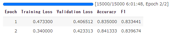
TrainOutput(global_step=15000, training_loss=0.406665673828125,
metrics={'train_runtime': 21710.6766, 'train_samples_per_second': 11.054,
'train_steps_per_second': 0.691, 'total_flos': 6.314722025472e+16,
'train_loss': 0.406665673828125, 'epoch': 2.0})
今回は、学習に6時間程度かかりました。
推論テスト
推論結果はpredictにより得ることができます。
preds_output = trainer.predict(dataset_encoded["validation"])
これを混同行列で可視化してみます。
import numpy as np
import matplotlib.pyplot as plt
from sklearn.metrics import ConfusionMatrixDisplay, confusion_matrix

y_preds = np.argmax(preds_output.predictions, axis=1)
y_valid = np.array(dataset_encoded["validation"]["label"])
labels = dataset_encoded["train"].features["label"].names

def plot_confusion_matrix(y_preds, y_true, labels):
    cm = confusion_matrix(y_true, y_preds, normalize="true")
    fig, ax = plt.subplots(figsize=(6, 6))
    disp = ConfusionMatrixDisplay(confusion_matrix=cm, display_labels=labels)
    disp.plot(cmap="Blues", values_format=".2f", ax=ax, colorbar=False)
    plt.title("Normalized confusion matrix")
    plt.show()

plot_confusion_matrix(y_preds, y_valid, labels)
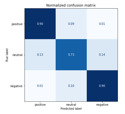
positive, negativeについては9割以上で正解できていますが、neutralの判別が少し難しくなっていそうです。 またpositiveをnegativeに間違えたり、negativeをpositiveに間違えたりすることは少ないようです。
モデル保存
保存前にラベル情報を設定しておきます。
id2label = {}
for i in range(dataset["train"].features["label"].num_classes):
    id2label[i] = dataset["train"].features["label"].int2str(i)

label2id = {}
for i in range(dataset["train"].features["label"].num_classes):
    label2id[dataset["train"].features["label"].int2str(i)] = i

trainer.model.config.id2label = id2label
trainer.model.config.label2id = label2id
保存先として、Google DriveをあらかじめColabにマウントしておきます。
そして、save_modelで保存します。
trainer.save_model(f"/content/drive/MyDrive/sample-text-classification-bert")
保存結果は以下のようなファイル構成となります。
sample-text-classification-bert
├── config.json
├── pytorch_model.bin
├── special_tokens_map.json
├── tokenizer_config.json
├── training_args.bin
└── vocab.txt
モデルやトークナイザの設定ファイル、そしてメインのモデルはpytorch_model.binとして保存されているようです。
ロードして推論
きちんと保存されているかテストします。
以下でPyTorchモデルとしてロードされます。
new_tokenizer = AutoTokenizer\
    .from_pretrained(f"/content/drive/MyDrive/sample-text-classification-bert")

new_model = (AutoModelForSequenceClassification
    .from_pretrained(f"/content/drive/MyDrive/sample-text-classification-bert")
    .to(device))
サンプルテキストを推論します。
inputs = new_tokenizer(sample_text, return_tensors="pt")

new_model.eval()

with torch.no_grad():
    outputs = new_model(
        inputs["input_ids"].to(device),
        inputs["attention_mask"].to(device),
    )
outputs.logits
tensor([[ 1.7906, 1.3553, -3.2282]], device='cuda:0')
logitsを推論ラベルに変換します。
y_preds = np.argmax(outputs.logits.to('cpu').detach().numpy().copy(), axis=1)
def id2label(x):
    return new_model.config.id2label[x]
y_dash = [id2label(x) for x in y_preds]
y_dash
['positive']
コードまとめ
ここまで色々とコードを書いてきましたが、以下にまとめを書いておきます。 まとめると非常にシンプルなコード量で実装できていることが分かります。
- インストール
!pip install transformers
!pip install datasets
!pip install fugashi # tokenizerが内部で使用
!pip install ipadic # tokenizerが内部で使用
- コード
from datasets import load_dataset
from transformers import AutoModelForSequenceClassification, AutoTokenizer
from transformers import TrainingArguments
from transformers import Trainer
from sklearn.metrics import accuracy_score, f1_score
from sklearn.metrics import ConfusionMatrixDisplay, confusion_matrix
import torch
import matplotlib.pyplot as plt
import numpy as np

# データセット取得
dataset = load_dataset("tyqiangz/multilingual-sentiments", "japanese")

# トークナイザの取得
tokenizer = AutoTokenizer.from_pretrained("cl-tohoku/bert-base-japanese-whole-word-masking")

# モデルの取得
device = torch.device("cuda" if torch.cuda.is_available() else "cpu")
num_labels = dataset["train"].features["label"].num_classes
model = (AutoModelForSequenceClassification
    .from_pretrained("cl-tohoku/bert-base-japanese-whole-word-masking", num_labels=num_labels)
    .to(device))

# トークナイザ処理
def tokenize(batch):
    return tokenizer(batch["text"], padding=True, truncation=True)
dataset_encoded = dataset.map(tokenize, batched=True, batch_size=None)

# トレーニング準備
batch_size = 16
logging_steps = len(dataset_encoded["train"]) // batch_size
model_name = f"sample-text-classification-distilbert"
training_args = TrainingArguments(
    output_dir=model_name,
    num_train_epochs=2,
    learning_rate=2e-5,
    per_device_train_batch_size=batch_size,
    per_device_eval_batch_size=batch_size,
    weight_decay=0.01,
    evaluation_strategy="epoch",
    disable_tqdm=False,
    logging_steps=logging_steps,
    push_to_hub=False,
    log_level="error",
)

# 評価指標の定義
def compute_metrics(pred):
    labels = pred.label_ids
    preds = pred.predictions.argmax(-1)
    f1 = f1_score(labels, preds, average="weighted")
    acc = accuracy_score(labels, preds)
    return {"accuracy": acc, "f1": f1}

# トレーニング
trainer = Trainer(
    model=model, args=training_args,
    compute_metrics=compute_metrics,
    train_dataset=dataset_encoded["train"],
    eval_dataset=dataset_encoded["validation"],
    tokenizer=tokenizer
)
trainer.train()

# 評価
preds_output = trainer.predict(dataset_encoded["validation"])

y_preds = np.argmax(preds_output.predictions, axis=1)
y_valid = np.array(dataset_encoded["validation"]["label"])
labels = dataset_encoded["train"].features["label"].names

def plot_confusion_matrix(y_preds, y_true, labels):
    cm = confusion_matrix(y_true, y_preds, normalize="true")
    fig, ax = plt.subplots(figsize=(6, 6))
    disp = ConfusionMatrixDisplay(confusion_matrix=cm, display_labels=labels)
    disp.plot(cmap="Blues", values_format=".2f", ax=ax, colorbar=False)
    plt.title("Normalized confusion matrix")
    plt.show()
plot_confusion_matrix(y_preds, y_valid, labels)

# ラベル情報付与
id2label = {}
for i in range(dataset["train"].features["label"].num_classes):
    id2label[i] = dataset["train"].features["label"].int2str(i)

label2id = {}
for i in range(dataset["train"].features["label"].num_classes):
    label2id[dataset["train"].features["label"].int2str(i)] = i

trainer.model.config.id2label = id2label
trainer.model.config.label2id = label2id

# 保存
trainer.save_model(f"/content/drive/MyDrive/sample-text-classification-bert")

# ロード
new_tokenizer = AutoTokenizer\
    .from_pretrained(f"/content/drive/MyDrive/sample-text-classification-bert")

new_model = (AutoModelForSequenceClassification
    .from_pretrained(f"/content/drive/MyDrive/sample-text-classification-bert")
    .to(device))

# サンプルテキストで推論
inputs = new_tokenizer(sample_text, return_tensors="pt")
new_model.eval()
with torch.no_grad():
    outputs = new_model(
        inputs["input_ids"].to(device),
        inputs["attention_mask"].to(device),
    )
y_preds = np.argmax(outputs.logits.to('cpu').detach().numpy().copy(), axis=1)
def id2label(x):
    return new_model.config.id2label[x]
y_dash = [id2label(x) for x in y_preds]
y_dash
まとめ
いかがでしたでしょうか?
かなりライブラリが整っているため、典型的なタスクであればすぐに試すことができそうな印象を受けました。 PyTorchなどのフレームワークの扱いは随所で必要になってくるため、前提としてそこら辺の知識はある程度求められそうです。 実用する場合などで自身でタスク用のヘッドを定義する場合は、よりPyTorchなどのフレームワークの知識は求められると思います。
まだまだ多くの機能やデータセットがあるので、今後他のタスクを実践してそちらも記事にできたらと思います。
本記事がHuggin Faceを使われる方の参考になれば幸いです。