Using Tableau’s Spatial Functions
この記事は公開されてから1年以上経過しています。情報が古い可能性がありますので、ご注意ください。
Introduction:
Tableau offers several spatial functions to improve data analysis. In this post, Tableau spatial functions are explained with examples.
Tableau Spatial Functions and how to use them:
There are several spatial functions which can be used in calculated fields or to join data sources. These are Area, Buffer, Distance, Makeline, Makepoint (using latitude and longitude) and Makepoint (using spatial reference identifier).
An important point to remember is that as of now, Tableau does not support mixed geometry in a single geospatial source, so if your data contains a mixture of different geometries such as: (points and polygons), or (points and lines), or (points and lines and polygons) then it is advisable to split your data according to the type of geometry and use the multilayered map feature to overlay such geometries on top of each other.
A brief explanation for the spatial functions along with the relevant examples are discussed below.
1. Area Function:
This function will calculate the total surface area of a spatial polygon. In case of line geometry or points geometry the area is returned with a value zero.
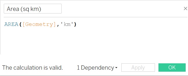
The syntax is, AREA(Polygon, "units"). Here “Polygon” is the column name which contains the geographic shape. For example, when using a shape file the column name is “Geometry”, however when using a hyper file containing geographic data the relevant column would be “Spatial Obj”. The “units” can be specified as meters ("meters" or "metres" or "m"), or kilometers ("kilometers" or "kilometres" or "km"), or miles ("miles" or "mi") or feet ("feet" or "ft").
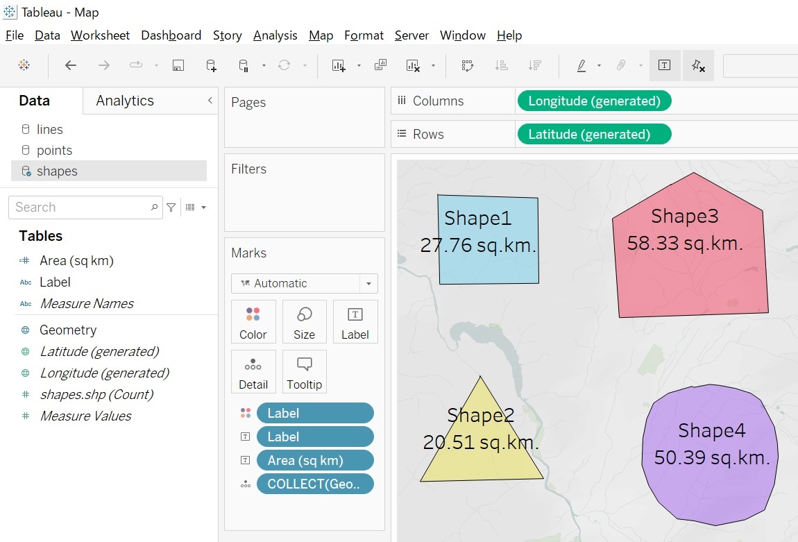
As an example, four custom shapes are introduced in Tableau using a shape file. Area of the polygons can be calculated with the following formula and its result is as shown below..
2. Buffer Function:
This function creates a buffer circle around a point in a specified unit and radial distance. This function will only work with point geometry datasource, if your datasource has lines or polygons this function will return an error.
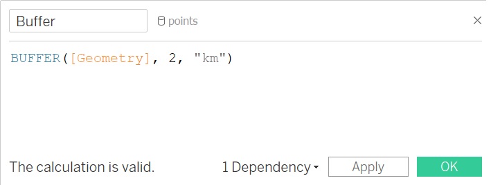
The syntax for this function is, BUFFER(Geometry, number, "units"). Here “Geometry” is the spatial field which contains points, “number” is the buffer circle’s radial distance and “units” can be specified as meters ("meters," "metres" "m"), or kilometers ("kilometers," "kilometres," "km"), or miles ("miles" or "mi"), feet ("feet," "ft"). This function can be created only with a live connection and it will continue to work when a data source is converted to an extract.
As an example, a datasource containing three spatial points is connected to Tableau and a calculated field “Buffer” is created as shown below. This field is automatically assigned a geographic role by Tableau.
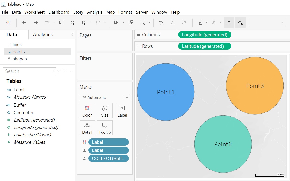
Plot the “Buffer” field on a map by double clicking on it, format the colors and labels to get a result as shown below.
3. Distance Function:
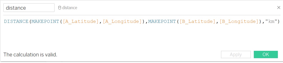
This function is used to calculate distance between two points. It works best with latitude and longitude data which is presented in a numbered format.
The syntax for this function is, DISTANCE(Point1, Point2, "units''). Here “Point1” and “Point2” are the points created using numeric latitude and longitude values from the data and “units” can be specified as meters ("meters," "metres" "m"), or kilometers ("kilometers," "kilometres," "km"), or miles ("miles" or "mi"), feet ("feet," "ft"). For example using this function distance can be calculated between two points, whose longitude value is 140 and latitude values are 35 and 36 as: DISTANCE(MAKEPOINT(35,140), MAKEPOINT(36,140), "km")
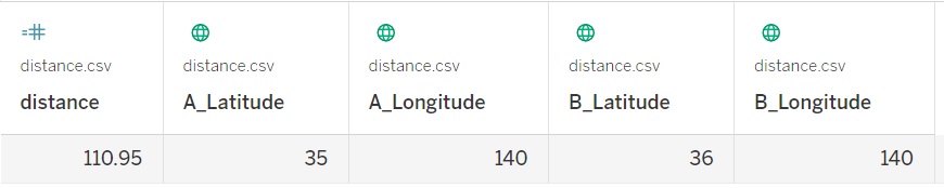
These points are fed to Tableau via a table and its corresponding distance calculation is as shown below:
4. Makeline Function:
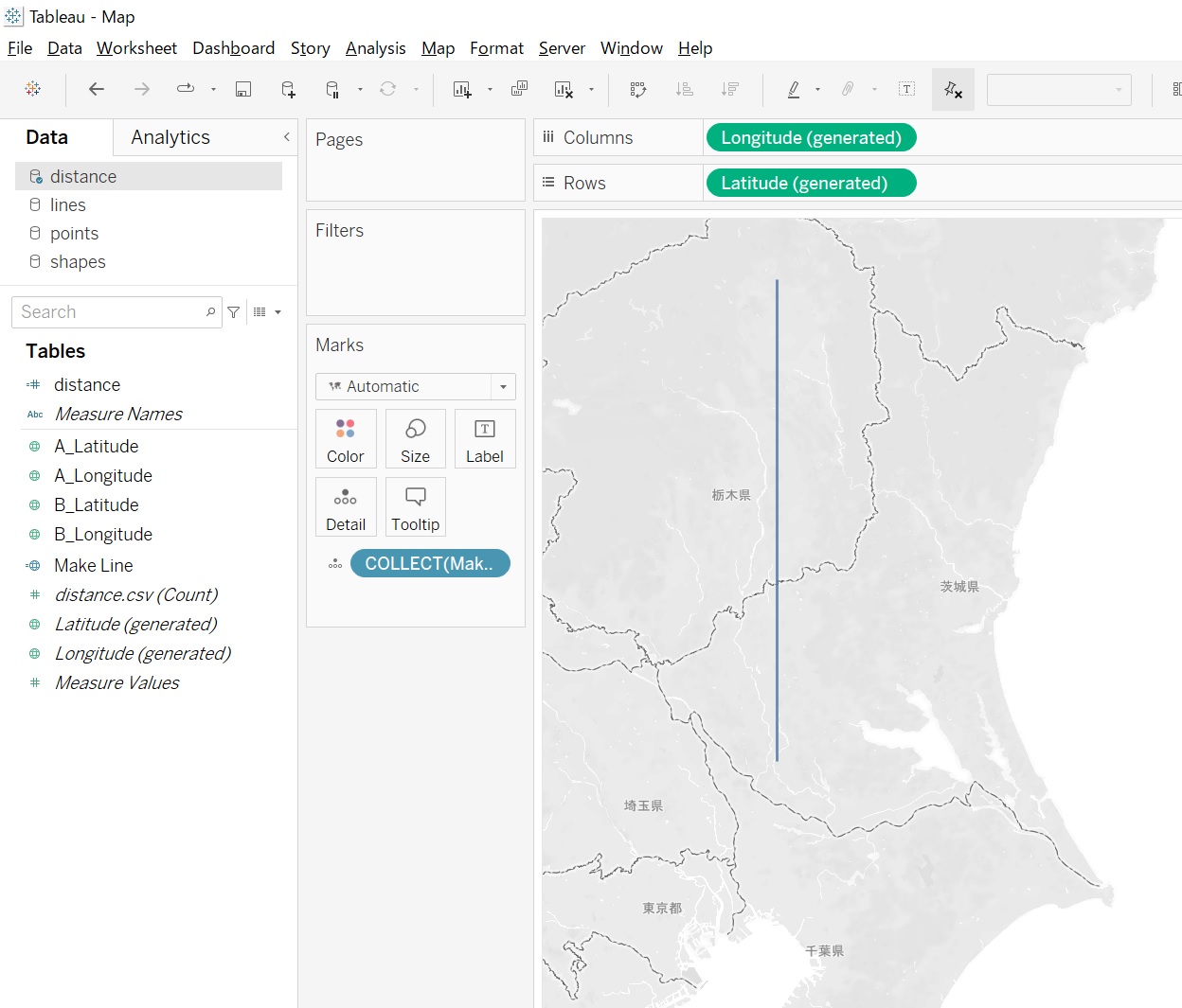
Use this function to generate a line between two points, it is helpful to build lines which have origin and destination on the maps. To plot multiple lines with just one calculated field, create multiple rows of data which have a pair of origin and destination points.
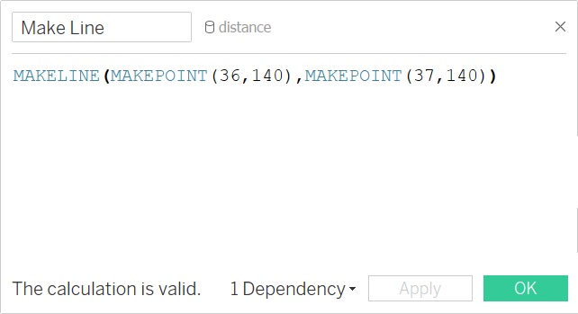
The syntax for this function is, MAKELINE(Point1, Point2). Here “Point1” and “Point2” are the points created using numeric latitude and longitude values from the data. For example using this function a line can be created between two points, whose longitude value is 140 and latitude values are 36 and 37 as:
Conversely, if the field is coming from the data then the formula can be changed to
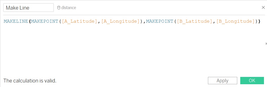
The results from such formula is depicted in the image below:
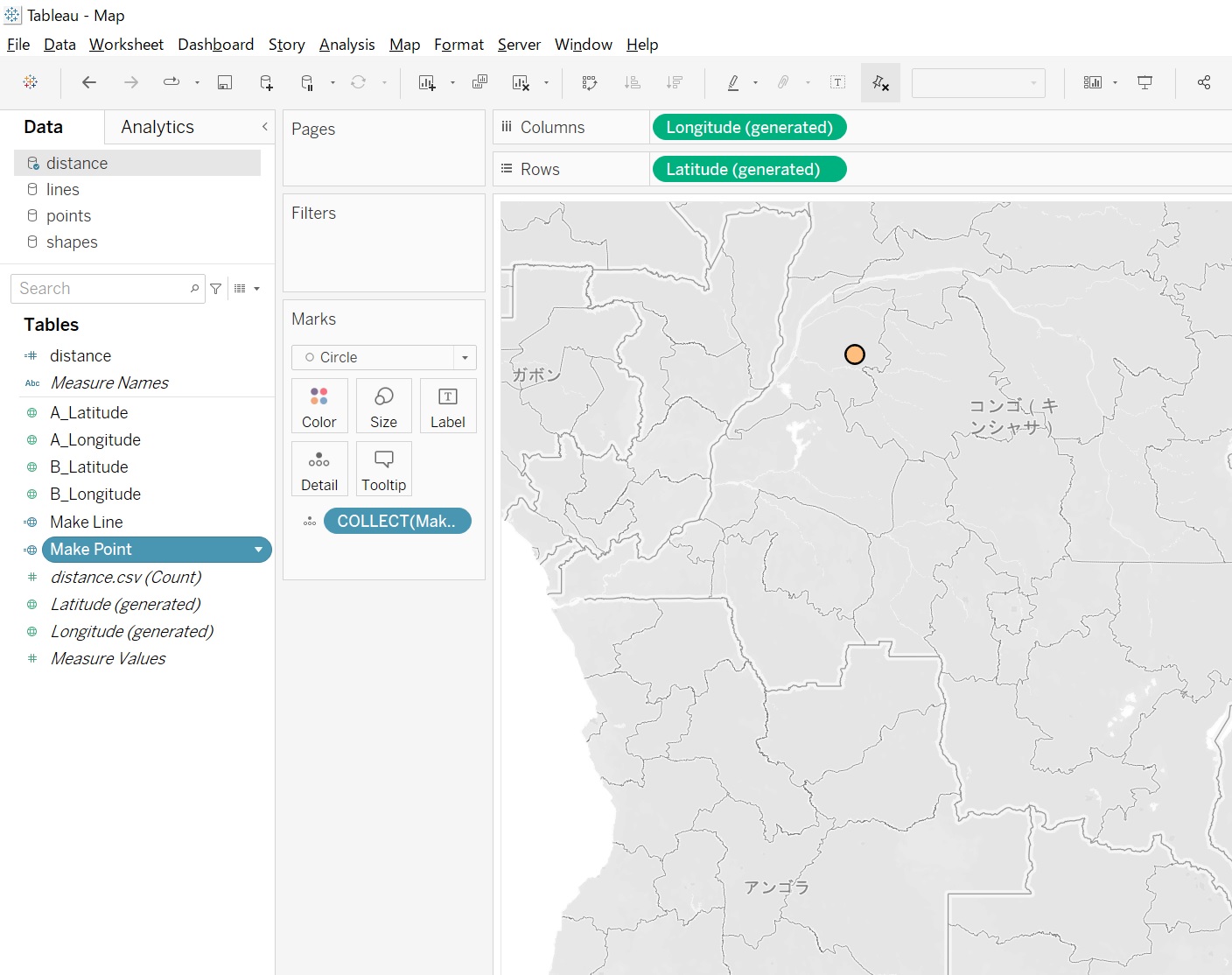
5. Makepoint Function using Latitude and Longitude:
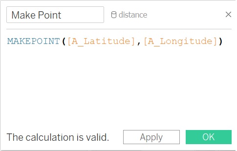
This formula will convert numeric data from latitude and longitude columns into spatial objects. MAKEPOINT can also be used to convert a non-spatial data source to be spatially-enabled so that it can be joined with another spatial file using a spatial join.
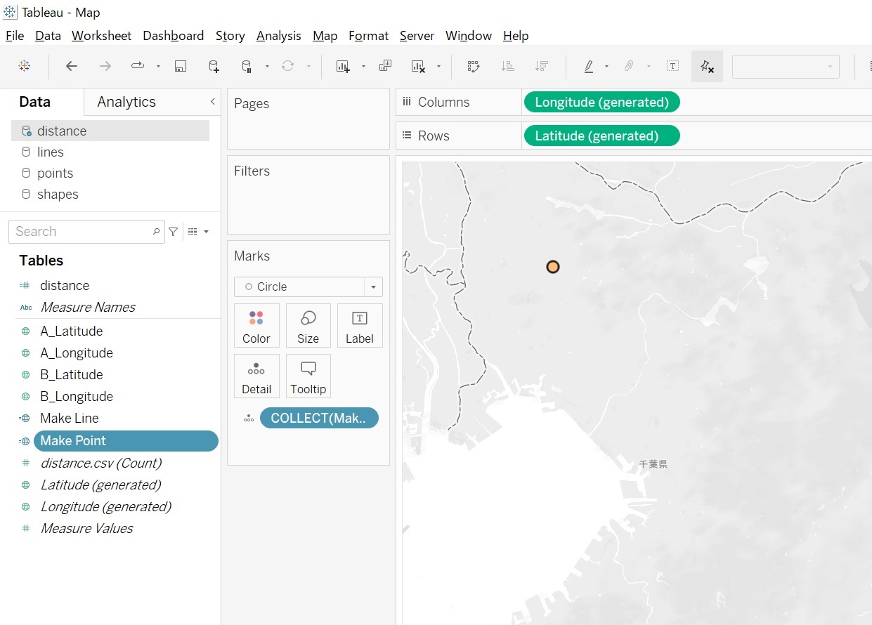
The syntax for this function is, MAKEPOINT(Latitude, Longitude). Here “Latitude” and “Longitude” are numeric values of latitudes and longitudes from the data. An example and its result is displayed below.
6. Makepoint Function using Spatial Reference Identifier:
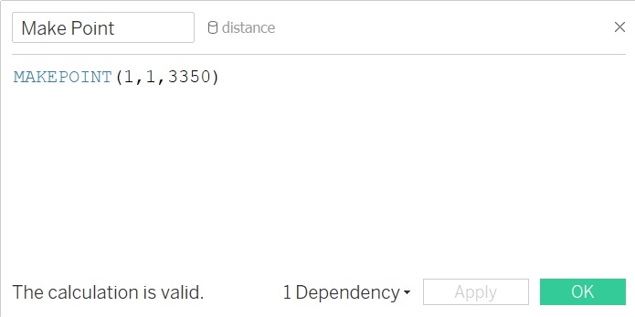
This formula can convert data from projected geographic coordinates to spatial objects. Spatial Reference Identifier (SRID) uses the EPSG reference system codes to specify coordinate systems. If SRID is not specified, WGS84 is assumed and parameters are treated as latitude/longitude in degrees by default. This function can only be created with a live connection and will continue to work when a data source is converted to an extract.
The syntax for this function is, MAKEPOINT(X-coordinate, Y-coordinate, SRID). An example and its result is displayed below.
Summary:
By using a variety of available spatial formulae, it is possible to do data analysis in Tableau.