Amazon SageMakerで産業用機械の温度データから異常値を検出してみた
この記事は公開されてから1年以上経過しています。情報が古い可能性がありますので、ご注意ください。
Amazon SageMakerはJupyterノートブックを使ったデータ探索から機械学習モデルの作成、エンドポイントの展開等が行える機械学習のフルマネージドサービスです。 今回はAmazon SageMakerの組み込みアルゴリズムであるランダムカットフォレスト(Random Cut Forest)を使用して、産業用機械の温度データから異常値の検出をしてみました。
※ 今回はノートブックインスタンス上ではなく、ローカル(macOS)環境のJupyterLab上で試しています。紹介する内容はノートブックインスタンスから実行しても動かない場合があります。試す際には適宜自身の環境に応じたものに置き換えるよう、お願いします。
ランダムカットフォレストについて
ランダムカットフォレストは決定木ベースのアンサンブル学習で主に異常検出に使われるアルゴリズムです。詳細については以下のエントリで解説されていますので、興味がある方はご覧ください。
使用するデータセットについて
今回使用するデータセットは産業用機械の温度データで、NAB(The Numenta Anomaly Benchmark)という異常検知のベンチマーク用ソフトウェアで使用されているものです。
やってみた
環境準備
まずは必要なモジュールをimportしておきます。不足しているモジュールがある場合はインストールが必要です。
import boto3
import sagemaker
from sagemaker.predictor import csv_serializer, json_deserializer
from sagemaker.estimator import Estimator
from sagemaker.amazon.amazon_estimator import get_image_uri
import pandas as pd
from urllib import request
import json
import math
import numpy as np
from tqdm import tqdm_notebook as tqdm
from more_itertools import chunked
import matplotlib.pyplot as plt
import seaborn as sns
データの保存場所の設定やセッションの作成等を行います。 環境に応じて書き換えてください。
# aws cliで登録しているプロファイル名とリージョン名を指定(ノートブックインスタンス上で有れば引数の指定は不要)
boto_sess = boto3.Session(profile_name='ml_pr', region_name='us-east-1')
sess = sagemaker.Session(boto_sess)

# データを保存するs3の場所を指定
bucket = 'bucket-name'
prefix = 'sagemaker/rcf-machine-temperature'

# 学習とエンドポイントの展開を行う際に使うIAMロール名(もしくはarn)
execution_role = 'iamrole-arn'
# ノートブックインスタンス上であればこちらのスクリプトでIAMロールを取得する
# execution_role = sagemaker.get_execution_role()

# pyplotで描画する図を綺麗にする
sns.set()

# 図がインラインで描画されるようにする(JupyterLabでは不要)
%matplotlib inline
データの取得
NABから産業用機械の温度データ(csv形式)を取得し、pandasのデータフレームとして読み込みます。合わせて、どのデータが異常値かを示すラベルデータ(json形式)も取得します。
# 対象のURLを指定
data_source = 'https://raw.githubusercontent.com/numenta/NAB/master/data/realKnownCause/machine_temperature_system_failure.csv'
label_data_source = 'https://raw.githubusercontent.com/numenta/NAB/master/labels/raw/known_labels_v1.0.json'

# 読み込み
df = pd.read_csv(data_source)
with request.urlopen(label_data_source) as f:
    label_data = json.loads(f.read().decode())

df
インデックスは行番号、列には日時(timestamp)と温度(value)があります。

データの前処理
学習の前にデータを扱いやすい形に加工します。 まずはインデックスをtimestampにして、データを見やすいようにします。
df.index = pd.to_datetime(df.timestamp)
df = df.drop(columns='timestamp')
異常値かどうかのラベルデータを列に追加します。
anomaly_dates = label_data['realKnownCause/machine_temperature_system_failure.csv']
anomaly_datetimes = [pd.to_datetime(dt) for dt in anomaly_dates]
is_anomaly = [int(timestamp in anomaly_datetimes) for timestamp in df.index]

df['is_anomaly'] = pd.Series(is_anomaly, index=df.index)
df[df.is_anomaly==1]
異常値である4つのデータポイントはこのようになっています。

異常値を黒丸として、データを描画してみます。
plt.figure().set_figwidth(10)
plt.plot(df.value, 'C0')
plt.plot(df[df.is_anomaly == 1].value, 'ko')
plt.show()

学習用とテスト用にデータを分割します。 今回は雑にデータの前半部分を学習用、後半部分をテスト用とします。 異常値はそれぞれのデータに2点ずつ含まれています。
bound = math.ceil(len(df)/2)
former_df = df.iloc[:bound]
later_df = df.iloc[bound:]
今回扱うのは時系列データなのでシングリング処理を施すことによって、温度変化を特徴量に含ませます。 産業用機械であれば1日ごとの周期性が含まれていそうなので、12(1時間のデータ数) * 24(時間数)=288個のデータを1つのデータポイントとして扱います。
def shingle(data, shingle_size):
    num_data = len(data)
    shingled_data = np.zeros((num_data-shingle_size, shingle_size))

    for n in range(num_data - shingle_size):
        shingled_data[n] = data[n:(n+shingle_size)]
    return shingled_data

shingle_size = 12 * 24
train_data = shingle(train_df.value, shingle_size)

# シングリングすることでシングルサイズ-1個のデータが無くなるので、データフレームも合わせておく
train_df_cut = train_df.iloc[shingle_size:]
テスト用データも学習用データと同様にシングリング処理を施します。加えて、テストデータには各行の先頭に異常値かどうかのラベルをつけます。
#テストデータも学習用データ同様に作成する
test_data = shingle(test_df.value, shingle_size)
test_df_cut = test_df.iloc[shingle_size:]

# ラベルをつける(異常値:1, 正常値:0)
labeled_test_data = [np.insert(row, 0, test_df_cut.is_anomaly[i]) for i, row in enumerate(test_data)]
データをS3に保存
学習用データをcsv形式でファイルに書き出し、s3にアップロードします。
train_local_path = './train.csv'
test_local_path = './test.csv'
train_s3_path = prefix+'/train.csv'
test_s3_path = prefix+'/test.csv'

# csv形式でファイル書き出し
np.savetxt(train_local_path, train_data, delimiter=',')
np.savetxt(test_local_path, labeled_test_data, delimiter=',')

# S3へアップロード
s3 = boto3.resource('s3')
s3.Bucket(bucket).upload_file(train_local_path, train_s3_path)
s3.Bucket(bucket).upload_file(test_local_path, test_s3_path)
学習
学習用データの場所や学習用インスタンスの設定、ハイパーパラメータの設定などを行います。
ml.m4.xlargeのインスタンス1台で学習します。
# ランダムカットフォレスト用のコンテナイメージ
training_image = get_image_uri(boto_sess.region_name, 'randomcutforest')

# 学習用処理の設定
rcf = Estimator(role=execution_role,
                    train_instance_count=1,
                    train_instance_type='ml.m4.xlarge',
                    output_path='s3://{}/{}/output'.format(bucket, prefix),
                    base_job_name='rcf-machine-temperature',
                    image_name=training_image,
                    sagemaker_session=sess)

# ハイパーパラメータの設定
rcf.set_hyperparameters(num_samples_per_tree=256,
                        num_trees=1000,
                        feature_dim=shingle_size)

# 教師データ
train_s3_data = sagemaker.s3_input(
   s3_data='s3://{}/{}'.format(bucket,train_s3_path),
   content_type='text/csv;label_size=0',
   distribution='ShardedByS3Key')
# テストデータ
test_s3_data = sagemaker.s3_input(
   s3_data='s3://{}/{}'.format(bucket,test_s3_path),
   content_type='text/csv;label_size=1',
   distribution='FullyReplicated')
学習を実行します。
rcf.fit({'train': train_s3_data, 'test': test_s3_data})
5分と経たずに学習ジョブが終わるはずです。マネジメントコンソールのSageMakerのジョブ詳細からログの表示でログを見ることができます。
今回はテストデータを入れているので、ログの最後にテストデータでの検証結果が表示されます。全てのデータポイントで異常値ではない判定されてしまったようで、negative_precisionが1にも関わらず、precisionは0になってしまいました。詳細についてはこのあとテストデータの異常度スコアを計算してみて確認します。

エンドポイントにモデルを展開
先ほど学習させたモデルをエンドポイントに展開します。今回は検証用なので、エンドポイントインスタンスはml.t2.large1台です。
predictor = rcf.deploy(
    initial_instance_count=1,
    instance_type='ml.t2.large'
)

predictor.content_type = 'text/csv'
predictor.serializer = csv_serializer
predictor.accept = 'application/json'
predictor.deserializer = json_deserializer
異常度スコアの計算
デプロイが完了したら、テストデータで異常度スコアを計算してみます。データ数が多いので100分割したものを順次エンドポイントに投げます。全ての計算が終わるまで約1分ほどかかります。
scores = []
chunk_size = math.ceil(len(test_data)/100)
for dat in tqdm(chunked(test_data, chunk_size)):
    results = predictor.predict(dat)
    for datum in results['scores']:
        scores.append(datum['score'])

# 異常度スコアを入れる
test_df_cut['score'] =  pd.Series(scores, test_df_cut.index)
BrokenPipeErrorが発生した時は...
データを分割せずにエンドポイントに投げようとしたら↓のようなBrokenPipeErrorが発生しました。 1行だけやデータを分割した場合であれば異常度スコアの計算に成功しました。なので、推論リクエストを投げたのにレスポンスが返って来ずにエラーが発生した場合には、タイムアウトしている可能性があるため、データを分割した上で推論リクエストを投げてみることをお勧めします。
BrokenPipeError: [Errno 32] Broken pipe

During handling of the above exception, another exception occurred:
ProtocolError: ('Connection aborted.', BrokenPipeError(32, 'Broken pipe'))

During handling of the above exception, another exception occurred:
ConnectionClosedError: Connection was closed before we received a valid response from endpoint URL: "https://runtime.sagemaker.us-east-1.amazonaws.com/endpoints/randomcutforest-2018-10-26-02-50-49-316/invocations".
異常度スコアの閾値を計算
どの程度の異常度スコアであれば異常であるかという判定を下すための閾値を計算します。今回は平均値から標準偏差の3倍の値が離れたところを閾値とします。
score_mean = test_df_cut.score.mean()
score_std = test_df_cut.score.std()
score_cutoff = score_mean + 3*score_std
test_df_cut['anomaly_threshold'] = pd.Series([score_cutoff]*len(test_df_cut), test_df_cut.index)
異常度スコアの確認
異常度スコアと元データを合わせてプロットします。
fig, ax1 = plt.subplots()
ax2 = ax1.twinx()

ax1.plot(test_df_cut.value, color='C0', alpha=0.7)
ax2.plot(test_df_cut.score, color='C1', alpha=0.7)

# 異常値のラベルデータ
anomalies_true = test_df_cut[test_df_cut.is_anomaly == 1]
ax1.plot(anomalies_true.value, 'ko' )

# 推論による異常値
anomalies_infer = test_df_cut.score[test_df_cut.score >= score_cutoff]
ax2.plot(anomalies_infer, 'ro' )
ax2.plot(test_df_cut.anomaly_threshold, 'r', alpha=0.5)

ax1.grid(which='major', axis='both')
ax1.set_ylabel('Machine Temperature', color='C0')
ax2.set_ylabel('Anomaly Score', color='C1')
ax1.tick_params('y', colors='C0')
ax2.tick_params('y', colors='C1')
ax1.set_ylim(0, max(test_df_cut.value))
ax2.set_ylim(min(test_df_cut.score), 1.5*max(max(test_df_cut.score), score_cutoff)+1)
fig.set_figwidth(12)
plt.show()

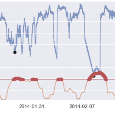
青い線が温度でオレンジの線が異常度スコアを表しています。青い線の上の黒丸は異常値のポイントです。赤い直線は異常度判定を下す閾値を示しています。残念ながらこの閾値設定では異常値であるはずのポイントにおいても、異常度スコアが閾値を超えることはありません。 とはいえ、異常値であるはずのポイントの異常度スコアが他の点に加えて上がってはいます。 ゆるい閾値設定(平均+1.5標準偏差)にすると異常値であるデータポイント付近を異常値判定出来るようになります。誤検出してしまっているポイントもあるので、閾値を決める際にはどの程度の異常値を検出したいかという要件のもとで決めると良さそうです。

エンドポイントの削除
必要な作業が終わったら、不要なコストがかからないようにエンドポイントを削除します。
predictor.delete_endpoint()
さいごに
Amazon SageMakerの組み込みアルゴリズムであるランダムカットフォレストを使って、産業用機械の温度の異常値検出を行いました。他の組み込みアルゴリズム同様簡単にできました。 学習時のテストデータの評価はよくない結果でしたが、推論した異常度スコアデータをプロットしたものを見てみると異常値のスコアは高くなっていることが分かりました。異常値を検出する要件によっては誤検出が含まれていたとしても、怪しいものはフラグを立てておくことも多いと思います。今回の場合もそういうケースと同様に、異常度スコアの閾値を下げることで誤検出を含めつつも異常値を検出する処理を作ったと考えると良いのかなと思います。
最後までお読み下さりありがとうございました〜!